论文解读（GraRep）《GraRep: Learning Graph Representations with Global Structural Information》

论文题目：《GraRep: Learning Graph Representations with Global Structural Information》
发表时间：  CIKM
论文作者：  Shaosheng Cao; Wei Lu;  Qiongkai Xu
论文地址：  Download
Github：      Go

---

Abstract

　　在本文中，我们提出了一种新的学习加权图顶点表示的GraRep模型。该模型学习低维向量来表示出现在图中的顶点，与现有的工作不同，它将图的全局结构信息集成到学习过程中。

---

1. Introduction

　　先引入 NE 的概念，然后介绍一下  DeepWalk ，但是作者抛出了一个问题，虽然  DeepWalk  确实有效果，但是为什么这么定义损失函数就可以得出效果呢？损失函数的可解释性并没有在  DeepWalk  论文中被谈及。

　　文中提到  skip-gram  模型其实就是用来量化两个节点的  $k$  阶关系（k-step relationship），所谓  $k$  阶关系就是两个顶点可以通过  $k$  步相连的关系。skip-gram  实际上是将节点之间的这种关系投影到一个平凡子空间（common subspace）中。而本文则是将k阶关系投影到独立的子空间（distict subspace）中。简单来说就是，skip-gram  模型将网络节点表示成向量后，节点的  $1$  到  $k$  阶关系全都综合反映到这个向量中。而GraRep则选择将  $1$  到  $k$  总共  $k$ 种关系分开，分别形成  $k$ 个向量，每个向量表示一种关系。

　　另一种方法 LINE，则是根本无法获取到  $k>2$  的节点关系。作者认为节点之间的  $k$  阶关系对把握网络的全局特征非常重要，越高阶的关系（也就是 $k$  越大）被考虑进来，得到的网络表示结果会越好。

　　本文的大致思路是通过矩阵分解的（matrix factorization）方法分别学习网络节点的  $k$  阶关系表示，然后将  $k$  个表示结合起来作为最终的表示结果。

　　总结一下贡献：

• • 提出学习图节点潜在向量表达的模型，能够捕获全局结构信息
  • 从概率观点对  DeepWalk  中同一采样的理解
  • 分析了负抽样相关的  Skip-Gram  模型的不足。

2. RELATED WORK

2.1 Linear Sequence Representation Methods

　　由 streams of words 组成的 Natural language corpora 可以看作是特殊的图结构，即  linear chains。目前，学习单词表征的方法有两种主要方法：neural embedding methods 和  matrix factorization based approaches 。

　　Neural embedding methods 采用 a fixed slide window 去捕捉当前单词的上下文词，例子：  skip-gram。

 　　虽然这些方法可能在某些任务上产生良好的性能，但由于它们使用单独的 local context windows ，而不是 global co-occurrence counts，因此它们在某些情况很差地捕获有用的信息。另一方面，矩阵分解的方法可以很好的利用  global statistics。

2.2 Graph Representation Approaches

　　经典的降维方法：

　　　　multidimensional scaling (MDS)、IsoMap 、LLE 、and Laplacian Eigenmaps 。

　　举例描述最近的一些 Graph Representation Approaches 。

3. Grarep model

3.1 Graphs and Their Representations

　　Definition 1. (Graph) A graph is defined as $G=(V, E)$. $V=\left\{v_{1}, v_{2}, \ldots, v_{n}\right\}$ is the set of vertices with each $V$ indicating one object while $E=\left\{e_{i, j}\right\}$ is the set of edges with each $E$ indicating the relationship between two vertices. A path is a sequence of edges which connect a sequence of vertices.

　　Some definitions：

• • $S$：adjacency matrix 。对于无权图：$S_{i, j}=1$ if and only if there exists an edge from $v_{i}$ to $v_{j}$, and $S_{i, j}=0$ otherwise。对于带权图：$S_{i, j}$ is a real number called the weight of the edge $e_{i, j}$ 。
  • $D$：diagonal matrix。

　　　　　　　　$D_{i j}= \begin{cases}\sum_{p} S_{i p}, & \text { if } i=j \\ 0, & \text { if } i \neq j\end{cases}$

　　定义从一个顶点  $v_i$  到  $v_j$  另一个顶点的转换概率，定义以下  (1-step) probability transition matrix ：

 　　　　$A=D^{-1} S$

　　该公式可以参考《邻接矩阵、度矩阵》

　　Definition 2. (Graph Representations with Global Structural Information) Given a graph $G$, the task of Learning Graph Representations with Global Structural Information aims to learn a global representation matrix $W \in \mathbb{R}^{|V| \times d}$ for the complete graph, whose $i$-th row $W_{i}$ is a $d$-dimensional vector representing the vertex $v_{i}$ in the graph $G$ where the global structural information of the graph can be captured in such vectors.

　　在本文中，全局结构信息有两个功能：

1. 1. the capture of long distance relationship between two different vertices
   2. the consideration of distinct connections in terms of different transitional steps.

　　为了验证这一点，Figure 1 给出了一些说明性的例子，说明了 k-step (对于 k=1、2、3、4 )关系信息的重要性，这些信息需要在顶点 A1 和 A2 之间捕获。

　　　　　　　　

　　

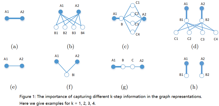
　　 Here, (a) and (e) show the importance of capturing the simple 1-step information between the two vertices which are directly connected to each other, where one has a stronger relation and the other has a weaker relation.

　　In (b) and (f), 2-step information is shown, where in (b) both vertices share many common neighbors, and in (f) only one neighbor is shared between them. Clearly, 2- step information is important in capturing how strong the connection between the two vertices is – the more common neighbors they share, the stronger the relation between them is.

　　In (c) and (g), the importance of 3-step information is illustrated. Specifically, in (g), despite the strong relation between  A1 and B, the relation between A1 and A2 can be weakened due to the two weaker edges connecting B and C, as well as C and A2. In contrast, in (c), the relation between A1 and A2 remains strong because of the large number of common neighbors between B and A2 which strengthened  their relation. Clearly such 3-step information is essential to be captured when learning a good graph representation with global structural information.

　　Similarly, the 4-step information can also be crucial in revealing the global structural properties of the graph, as illustrated in (d) and (h). Here, in (d), the relation between A1 and A2 is clearly strong, while in (h) the two vertices are unrelated since there does not exist a path from one vertex to the other. In the absence of 4-step relational information, such important distinctions can not be properly captured.

　　总结：一阶邻居带来的信息很重要，k-step 之间的邻居信息受到中间邻居之间的影响。

　　现在思考是否考虑对不同的 k-step 进行区别对待？当然。

　　　　　　

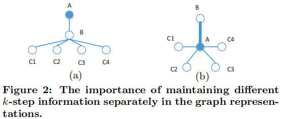
　　我们认为，在学习图表示时，区别对待不同的  k-step  信息是必要的。我们在 Figure 2 的 (a) 中提供了一个简单的图。让我们重点学习图中  A  顶点的表示。我们可以看到， A  在学习其表示时接收到两种类型的信息：来自  B  的 1-step 信息，以及来自所有  C  顶点的  2-step  信息。我们注意到，如果我们不区分这两种不同类型的信息，我们可以构建一个替代图，如 Figure 2 中的(b)所示，其中  a  接收的信息与 (a) 完全相同，但具有完全不同的结构。

3.2 Loss Function On Graph

　　现在考虑从顶点  $w$  到顶点 $c$  ,设从顶点  $w$  到顶点 $c$ 的概率转移为 $p_{k}(c \mid w)$。我们已经知道  $1-step$  是什么，为了计算 $k-step$ ，我们引入了下面的  k-step probability transition matrix：

　　　　$A^{k}=\underbrace{A \cdots A}_{k}$

　　 我们可以观察到，$A_{i, j}^{k}$  恰好是指从顶点 $i$  到顶点  $j$  的转移概率，其中转移恰好由  $k$ 步组成。这将直接导致：

　　　　$p_{k}(c \mid w)=A_{w, c}^{k}$

　　其中，  $A_{w, c}^{k}$  是矩阵  $ A^{k}  $  的第  $w$  行和第  $c$  列中的元素。.

　　那么优化目标就是：对于任意的一个  $(w,c)$  的组合，最大化这个组合所代表的路径在图中的概率，最小化除了这个组合外在图中的概率。换句话说，对于所有的  $(w,c)$   组合对，如果   $(w,c)$  所代表的路径在图中，那么增大它的概率；如果  $(w,c)$   所代表的路径不在图中，那么减小它的概率。

　　本文使用了 NCE 损失函数来反应这种特性，损失函数的定义是：

　　　　$L_{k}=\sum \limits _{w \in V} L_{k}(w)$

　　其中 

　　　　$L_{k}(w)=\left(\sum \limits _{c \in V} p_{k}(c \mid w) \log \sigma(\vec{w} \cdot \vec{c})\right)+\lambda \mathbb{E}_{c^{\prime} \sim p_{k}(V)}\left[\log \sigma\left(-\vec{w} \cdot \vec{c}^{\prime}\right)\right]  \quad \quad \quad  (1)$ 

　　　　$\sigma(x)=\left(1+e^{-x}\right)^{-1}$ ；

　　　　$\lambda$ 是一个表示负样本数量的超参数；

　　　　$p_{k}(V) $ 是图中顶点上的分布；

　　　　$\mathbb{E}_{c^{\prime} \sim p_{k}(V)}[\cdot]$ 是当  $c^{\prime}$  遵循  $p_{k}(V) $  分布时的期望值；

 　　　   $c^{\prime}$ 是通过  negative sampling  获得的；

　　对于  $(1) $ 式：

• • 前项中的 $\sigma(\vec{w} \cdot \vec{c})$ 理解为 Graph 中节点对 $(w,c)$ 共同出现的概率，要最大化这个值。
  • 后项中的 $\sigma(-\vec{w} \cdot \vec{c})$  理解为 对于任意选取的节点  $c^{\prime}$  所形成的  $(w,c^{\prime})$  要最小化其出现的概率，最小化其出现概率就是最大化  $\sigma(-\vec{w} \cdot \vec{c})$  。

　　对于 $(1) $  式后项negative sampling 部分中的 $\mathbb{E}_{c^{\prime} \sim p_{k}(V)}\left[\log \sigma\left(-\vec{w} \cdot \overrightarrow{c^{\prime}}\right)\right]$

　　　　$=p_{k}(c) \cdot \log \sigma(-\vec{w} \cdot \vec{c})+\sum \limits _{c^{\prime} \in V \backslash\{c\}} p_{k}\left(c^{\prime}\right) \cdot \log \sigma\left(-\vec{w} \cdot \overrightarrow{c^{\prime}}\right)   \quad \quad \quad  (2)$

　　对于  $(2) $ 式：

• • $p_{k}(V)$  是网络中节点的概率分布。negative sampling 部分实际上就是节点  $c^{\prime}$  服从  $p_{k}(V)$  分布时 $(w,c)$ 不出现的期望。对于随机采样的一个节点  $c^{\prime}$  ，如果正好选到了正确的节点  $c$，那么对应的就是  $(2) $  中前项；如果没有选到  $c$ ，那么对应的就是  $(2) $  中后项。因此对于一个特定的  $(w,c)$ 组合对来说，损失函数表达如下：

　　　　　　$L_{k}(w, c)=p_{k}(c \mid w) \cdot \log \sigma(\vec{w} \cdot \vec{c})+\lambda \cdot p_{k}(c) \cdot \log \sigma(-\vec{w} \cdot \vec{c})\quad \quad \quad  (3)$

　　文中提到：随着  $k$  的增长，$w$  经过  $k$  步到达  $c$  的概率会逐渐收敛到一个固定值。　　

　　计算  $p_{k}(c)$ ：任一节点经过  $k$  步到达节点  $c$  的概率，因此等于所有  $k$  步可以到达  $c$  的路径的概率加和。

　　　　$p_{k}(c)=\sum \limits _{w^{\prime}} q\left(w^{\prime}\right) ,  \quad p_{k}\left(c \mid w^{\prime}\right)=\frac{1}{N} \sum \limits_{w^{\prime}} A_{w^{\prime}, c}^{k}$

 　　其中：

　　　　$q^{\prime}(\omega)=\frac{1}{N}, \quad p_{k}(c \mid \omega^{\prime})=A_{\omega^{\prime}, c}^{k}$

　　　　$N$ 是图  $G$ 中的顶点数。

　　　　$q(w^{\prime})$ 为选择  $w^{\prime}$  作为路径中的第一个顶点的概率，这里假设为均匀分布。

　　将  $p_{k}(c \mid w), \quad p_{k}(c)$  代入 $(3)$  式得到：

 　　　　$L_{k}(w, c)=A_{w, c}^{k} \cdot \log \sigma(\vec{w} \cdot \vec{c})+\frac{\lambda}{N} \sum \limits _{w^{\prime}} A_{w^{\prime}, c}^{k} \cdot \log \sigma(-\vec{w} \cdot \vec{c})\quad \quad \quad  (4)$

　　我们令  $e=\vec{w} \cdot \vec{c}$  ，对   $L_{k}(w) $  求偏导，并令   $\frac{\partial L_{k}}{\partial e}=0$  

　　推导过程如下：

　　　　令   $x=\vec{w} \cdot \vec{c}$,   $A_{w^{\prime}, c}^{k}=A$,   $\frac{\lambda}{N} \sum_{w^{\prime}} A_{w^{\prime}, c}^{k}=B$ 

　　　　那么 $L_{k}=A \log \sigma(x)+B \log \sigma(-x)$

　　　　　　$\frac{\partial L_{k}}{\partial x}=A \cdot \frac{\sigma^{\prime}(x)}{\sigma(x)}+B \frac{-\sigma^{\prime}(-x)}{\sigma(-x)}=A \frac{\sigma(x)(1-\sigma(x))}{\sigma(x)}-B \cdot \frac{\sigma(-x)(1-\sigma(-x))}{\sigma(-x)}$

　　　　　　$\begin{aligned}&=A \cdot(1-\sigma(x))-B(1-\sigma(-x)) \\&=A\left(1-\frac{1}{1+e^{-x}}\right)-B\left(1-\frac{1}{1+e^{x}}\right) \\&=A \cdot \frac{e^{-x}}{1+e^{-x}}-B \frac{e^{x}}{1+e^{x}} \\&=A \frac{1}{e^{x}+1}-B \frac{e^{x}}{1+e^{x}}=0 . \\&e^{x} =\frac{A}{B} ,\quad x=\log \frac{A}{B}=\log \frac{ A_{w^{\prime} , c}^{k}}{\sum \limits _{w^{\prime}} A_{w^{\prime} , c}^{k}}-\log \frac{\lambda}{N}\end{aligned}$

　　最终得到：

　　　　$\vec{w} \cdot \vec{c}=\log \left(\frac{A_{w, c}^{k}}{\sum \limits _{w^{\prime}} A_{w^{\prime}, c}^{k}}\right)-\log (\beta)$

　　其中  $\beta = \frac{\lambda}{N} $。

　　这得出结论，我们基本上需要将矩阵 $Y$ 分解成两个矩阵  $ W$  和  $C$  ，其中  $W$  的每一行和  $C$  的每一行分别由顶点  $w$  和  $c$  的向量表示组成，$Y$  的条目为：

　　之前的工作是为了找到这样一个矩阵  $Y$  ，它编码了网络中所有节点相互之间的关系，但是这个矩阵的维数很高（$|V| \times |V| $），不能直接用来作为网络的表示。因此要用矩阵分解的方法对  $Y$  进行分解，分解后形成的  $W、C$  矩阵维数要远远小于  $Y$  的维度，其中  $W$  的每一行和  $C$  的每一行分别由顶点  $w$  和  $c$  的向量表示组成，而这个  $W$  矩阵就是网络节点的表示，$C$  矩阵就是上下文节点的表示（不关心这个矩阵）：

　　　　$Y_{i, j}^{k}=W_{i}^{k} \cdot C_{j}^{k}=\log \left(\frac{A_{i, j}^{k}}{\sum \limits _{t} A_{t, j}^{k}}\right)-\log (\beta)$

3.3 Optimization with Matrix Factorization

　　为了降低误差，将矩阵  $Y$  中负值全被替换为  $0$ ，形成一个新的矩阵  $X$ ：

　　　　$X_{i, j}^{k}=\max \left(Y_{i, j}^{k}, 0\right)$

 　　这里采用  $SVD$  分解，矩阵  $X$   被分解为：

　　　　$X^{k}=U^{k} \Sigma^{k}\left(V^{k}\right)^{T}$

　　其中  $U$  和  $V$  是正交矩阵，$Σ$  是由奇异值的有序列表组成的对角矩阵。

　　接下来用SVD方法将矩阵  $X$  分解成：

　　　　$X^{k}=U^{k} \Sigma^{k}\left(V^{k}\right)^{T}$

　　因为最终的网络表示要求是  $d$  维的，那么进一步将  $X$  分解为：

　　　　$X^{k} \approx X_{d}^{k}=U_{d}^{k} \Sigma_{d}^{k}\left(V_{d}^{k}\right)^{T}$

　　其中：$\Sigma_{d}^{k}$  是由 top  d  奇异值组成 的，而且 $U_{d}^{k}$  和   $V_{d}^{k}$  分别是  $U^{k}$  和  $ V^{k}$ 前  $d$  列组成。

　　最后得到：

　　　　$X^{k} \approx X_{d}^{k}=W^{k} C^{k}$

　　其中：

　　　　$W^{k}=U_{d}^{k}\left(\Sigma_{d}^{k}\right)^{\frac{1}{2}}, \quad C^{k}=\left(\Sigma_{d}^{k}\right)^{\frac{1}{2}} V_{d}^{k T}$

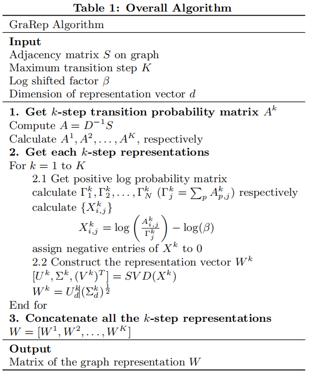
4. Algorithm

　　Step 1. Get  $k-step$ transition probability matrix  $A_k$  for each  $k = 1, 2, . . . , K$.

　　Step 2. Get each  $k-step$  representation

　　Step 3. Concatenate all  $k-step$  representations

　　　　　　　　

CONCLUSIONS

　　除了公式多，其他没啥...............那天心情好了补完。

　　更多内容可以参考

　　https://zhuanlan.zhihu.com/p/46446600

　　https://blog.csdn.net/weixin_40675092/article/details/118225889

『总结不易，加个关注呗！』