神经网络

目录

• 1 全连接层的实现
  • 1.1手动创建的方式
  • 1.2 自动创建的方式：高层接口
  • 1.2 网络层的参数总结
• 2 前向传播(隐层层的设计)
• 3 激活函数
  • 3.1 sigmoid函数
    • 3.1.1表达式
    • 3.1.2 图像
    • 3.1.3 函数接口
    • 3.1.4实例
  • 3.2 ReLU
    • 3.2.1 表达式
    • 3.2.2 图像
    • 3.2.3函数接口
    • 3.2.4 实例
  • 3.3 LeakyReLu
    • 3.3.1 表达式
    • 3.3.2图像
    • 3.3.3函数接口
    • 3.3.4实列
  • 3.4 Tanh
    • 3.4.1 表达式
    • 3.4.2图像
    • 3.4.3 函数接口
    • 3.4.4实例
  • 3.5 softmax
    • 3.5.1 表达式
    • 3.5.2图像
    • 3.5.3函数接口
    • 3.5.4实例
• 4 输出层的设计
• 5 误差函数
  • 5.1均方差
  • 5.2 交叉熵
• 6神经网络类型
• 7项目实战
  • 7.1 导入必要的库
  • 7.1读取数据集
  • 7.2 数据集预处理
    • 7.2.1 缺失值
    • 7.2.2 特殊列处理
    • 7.2.3 标准化
      • 7.2.3.1 划分训练集和测试集
      • 7.2.3.2 分离标签
      • 7.2.3.4 计算训练集的统计特性
      • 7.2.3.5 标准化
  • 7.3 批量化切分数据集
  • 7.4 构造神经网络
  • 7.5 选择优化器
  • 7.6 训练和测试
  • 7.7 作图

1 全连接层的实现

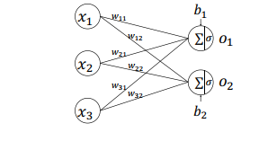
1.1手动创建的方式

import  tensorflow as tf
#输入是两个两本，每个样本的特征长度是3,输出分类为2
x = tf.random.normal([2, 3])
w = tf.Variable(tf.random.truncated_normal([3, 2],stddev=1))
b = tf.Variable(tf.random.truncated_normal([2]))

o1 = tf.matmul(x, w)+b

o2 = tf.nn.relu(o1)  #relu激活函数

print(o2)

out

tf.Tensor(
[[0.        0.       ]
[2.5625916 2.5094762]], shape=(2, 2), dtype=float32)

1.2 自动创建的方式：高层接口

layers.Dense(units, activation)，只需要指定输出节点数 Units 和激活函数类型即可

import tensorflow as tf
from tensorflow.keras import layers

x = tf.random.normal([4,100])
# 创建全连接层，指定输出节点数和激活函数
fc = layers.Dense(6,activation=tf.nn.relu)
# 通过 fc 类完成一次全连接层的计算
h1 = fc(x)
print(h1)
print(fc.kernel)#w
print(fc.bias)#b
print(fc.trainable_variables)#w和b

利用网络层类对象进行前向计算时，只需要调用类的__call__方法即可，即写成 fc(x)方式，它会自动调用类的__call__方法，在__call__方法中自动调用 call 方法， 全连接层类在 call 方法中实现了𝜎(𝑋@𝑊 + 𝒃)的运算逻辑， 最后返回全连接层的输出张量。

out

#输出的分类结果
tf.Tensor(
[[0.7934056  0.        ]
 [0.24560195 0.        ]
 [0.82438886 0.        ]
 [0.899623   0.        ]], shape=(4, 2), dtype=float32)
 #全连接层的权重w：fc.kernel
<tf.Variable 'dense/kernel:0' shape=(3, 2) dtype=float32, numpy=
array([[ 0.39674175, -0.2645977 ],
       [ 0.63121116, -1.0027896 ],
       [ 0.21580482, -0.31935608]], dtype=float32)>
#全连接层的偏置b:fc.bias
<tf.Variable 'dense/bias:0' shape=(2,) dtype=float32, numpy=array([0., 0.], dtype=float32)>

#w和b:fc,trainable_variables
[<tf.Variable 'dense/kernel:0' shape=(3, 2) dtype=float32, numpy=
array([[-0.563206  ,  0.39795756],
       [ 0.64601564,  0.04851365],
       [-0.42996007, -0.25872254]], dtype=float32)>, <tf.Variable 'dense/bias:0' shape=(2,) dtype=float32, numpy=array([0., 0.], dtype=float32)>]

上述通过一行代码即可以创建一层全连接层 fc， 并指定输出节点数为 2， 输入的节点数3,在fc(x)计算时自动获取， 并创建内部权值矩阵 W 和偏置 b。 我们可以通过类内部的成员名kernel 和 bias 来获取权值矩阵 W 和偏置 b：

1.2 网络层的参数总结

参数	函数函数接口	描述
w	fc.kernel	待优化权重参数
b	fc.bias	待优化偏置参数
w和b	fc.trainable_variables
batchnormali'za'ti'o'n的参数	fc.non_trainable_variables	不参与梯度优化的张量，如BatchNormalization 层
所有参数	fc.variables	所有参数列表

2 前向传播(隐层层的设计)

把神经网络从输入到输出的计算过程叫做前向传播(Forward propagation)。

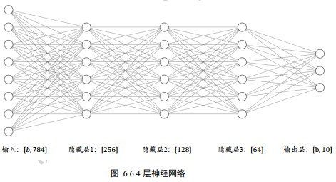
model = keras.Sequential([
    layers.Dense(512, activation=tf.nn.relu),
    layers.Dense(256, activation=tf.nn.relu),
    layers.Dense(64, activation=tf.nn.relu),
    layers.Dense(10,activation=None)
    ])
x = tf.random.normal([2,784],stddev=1)
out = model(x)
print(out)

3 激活函数

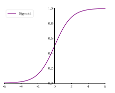
3.1 sigmoid函数

3.1.1表达式

sigmoid = 1/(1+e^-x)

3.1.2 图像

3.1.3 函数接口

tf.nn.sigmoid()

3.1.4实例

x = tf.linespace(-6.,6.,10)
print("befor:",x)
x1 = tf.nn.sigmoid(x)
print("after: ",x1)

out

before: tf.Tensor([-6.     -4.6666665 -3.3333333 -2.  -0.6666665  0.6666672.   3.333334   4.666667   6. ], shape=(10,),dtype=float32)

after:  tf.Tensor([0.00247262 0.00931596 0.0344452  0.11920292 0.33924365 0.6607564 0.880797   0.96555483 0.99068403 0.9975274 ], shape=(10,), dtype=float32)

可以看到，向量的范围由[-6,6]映射到[0,1]的区间。

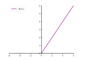
3.2 ReLU

在 ReLU(REctified Linear Unit， 修正线性单元)激活函数提出之前， Sigmoid 函数通常是神经网络的激活函数首选。 但是 Sigmoid 函数在输入值较大或较小时容易出现梯度值接近于 0 的现象， 称为梯度弥散象， 网络参数长时间得不到更新， 很难训练较深层次的网络模型

3.2.1 表达式

ReLU(X) = max(0,x)

3.2.2 图像

3.2.3函数接口

tf.nn.relu()

3.2.4 实例

x2 = tf.nn.relu(x)
print(x2)

out

tf.Tensor([0.  0.  0. 0.   0.   0.666667 2.    3.333334 4.666667 6.  ], shape=(10,), dtype=float32)

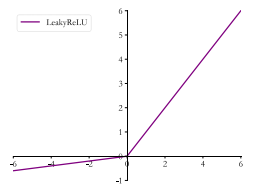
3.3 LeakyReLu

ReLU 函数在𝑥 < 0时梯度值恒为 0，也可能会造成梯度弥散现象，为了克服这个问题， LeakyReLU被提出。

3.3.1 表达式

$$
LeakyReLU=\begin{cases} x，x\geq0\ \alpha*x， x\leq0\end{cases}
$$

markdown 数学公式： https://blog.csdn.net/mingzhuo_126/article/details/82722455

3.3.2图像

3.3.3函数接口

tf.nn.leaky_relu(x,alpha=)

3.3.4实列

x3 = tf.nn.leaky_relu(x,alpha=0.1)
print(x3)

out

tf.Tensor([-0.6   -0.46666667 -0.33333334 -0.2    -0.06666666  0.666667
  2.      3.333334   4.666667    6. ], shape=(10,), dtype=float32)

tf.nn.leaky_relu 对应的类为 layers.LeakyReLU，可以通过LeakyReLU(alpha)创建 LeakyReLU 网络层，并设置a
参数，像 Dense 层一样将 LeakyReLU层放置在网络的合适位置

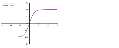
3.4 Tanh

3.4.1 表达式

$$
tanh(x)=(e^x-e)\div(e^x+e{-x})=2*sigmoid(2x)-1
$$

3.4.2图像

​

3.4.3 函数接口

tf.nn.tanh(x)

3.4.4实例

x4 = tf.nn.tanh(x)
print(x4)

out

tf.Tensor([-0.99998784 -0.99982315 -0.9974579  -0.9640276  -0.58278286  0.58278316
  0.9640276   0.99745804  0.99982315  0.99998784], shape=(10,), dtype=float32)

可以看到向量的范围被映射到[-1,1]之间 ,存在的问题如同sigmoid函数，可能出现梯度弥散

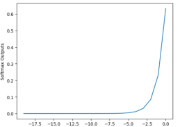
3.5 softmax

3.5.1 表达式

$$
\delta(z_i)=e^{{z_i}/\sum_{j=1}}{e^{z_j}}
$$

3.5.2图像

3.5.3函数接口

tf.nn.softmax()

layers.Softmax(axis=?)

与 Dense 层类似， Softmax 函数也可以作为网络层类使用， 通过类 layers.Softmax(axis=-1)
可以方便添加 Softmax 层，其中 axis 参数指定需要进行计算的维度 .

一般和交叉熵连用，不单独用：tf.keras.losses.categorical_crossentropy(y_true,y_pred,from_logits=False)

当 from_logits 设置为 False 时， y_pred 表示为经过 Softmax 函数的输出。

#实例
out = tf.random.normal([2,10])
y = tf.constant([1,3])
y_true = tf.one_hot(y,depth=10)
loss = tf.keras.losses.categorical_crossentropy(y_true,out,from_logits=True)#不使用softmax
print(loss)
loss = tf.reduce_mean(loss)#计算所有样本的平均交叉熵误差
print(loss)

out

tf.Tensor([0.86137515 1.7536191 ], shape=(2,), dtype=float32)
tf.Tensor(1.3074971, shape=(), dtype=float32)

3.5.4实例

x5 = tf.nn.softmax(x,axis=-1)
print(x5)
print(x5.numpy().sum())

out

tf.Tensor(
[4.5246225e-06 1.7164926e-05 6.5118009e-05 2.4703602e-04 9.3717279e-04
 3.5553228e-03 1.3487710e-02 5.1167924e-02 1.9411404e-01 7.3640400e-01], shape=(10,), dtype=float32)
1.0  #和为1

4 输出层的设计

输出层的设计，它除了和所有的隐藏层一样，完成维度变换、特征提取的功能，还作为输出层使用，需要根据具体的任务场景来决定是否使用激活函数，以及使用什么类型的激活函数。

输出空间	描述	适用问题	激活函数	误差计算
𝒐 ∈ 𝑅	输出属于整个实数空间，或者某段普通的实数空间	回归问题：年龄的预测、 股票走势的预测	无	均方差
𝒐 ∈ [0,1]	输出值特别地落在[0, 1]的区间	二分类问题，正反面问题	sigmoid	交叉熵/均方差
𝒐 ∈ [0,1],sum(oi)=1	输出值特别地落在[0, 1]的区间，并且所有输出值的和为1	多分类问题，MNIST	softmax	交叉熵
𝒐 ∈ [-1,1]	输出值在[-1,1]之间		tanh	交叉熵/均方差

5 误差函数

函数	适用对象	函数接口
均方差	回归问题	keras.losses.MSE(y_onehot, o) # 计算均方差
交叉熵	分类问题	tf.keras.losses.categorical_crossentropy(y_true,y_pred,from_logits=False)

5.1均方差

$$
MSE = 1/N\sum_{i=1}^{{N}{(y_i-o_i)}2}
$$

5.2 交叉熵

$$
H(p,q) = -\sum_{i=0}^{n}p(i)log_2q(i)
$$

6神经网络类型

卷积神经网络(CNN)

循环神经网络(RNN)

注意力网络(ATTENTION)

图神经网络(GCN)

7项目实战

利用全连接网络完成汽车的效能指标 MPG 的回归问题预测

7.1 导入必要的库

import tensorflow as tf
import pandas as pd
from tensorflow import keras
import os
import seaborn as sns
import matplotlib.pyplot as plt
import pathlib
from tensorflow.keras import layers, datasets, optimizers, losses

7.1读取数据集

我们采用 Auto MPG 数据集，它记录了各种汽车效能指标与气缸数、重量、马力等其他因子的真实数据， 查看数据集的前 5 项，如表格 6.1 所示，其中每个字段的含义列在表格 6.2 中。除了产地的数字字段表示类别外，其他字段都是数值型。对于产地地段， 1 表示美国， 2 表示欧洲， 3 表示日本

dataset_path = keras.utils.get_file("auto-mpg.data", \
 "http://archive.ics.uci.edu/ml/machine-learning-databases/auto-mpg/auto-mpg.data")
 
 #原始数据没有title，给数据类型添加title
column_names = ['MPG', 'Cylinders', 'Displacement', 'Horsepower', 'Weight',
                'Acceleration', 'Model Year', 'Origin']

raw_dataset = pd.read_csv(dataset_path, names=column_names, \
                          na_values="?", comment='\t', sep=" ", \
                          skipinitialspace=True)
dataset = raw_dataset.copy()

查看数据集

print(dataset.head())

    MPG     Cylinders    Displacement  ...  Acceleration  Model Year  Origin
0  18.0          8         307.0  ...          12.0          70       1
1  15.0          8         350.0  ...          11.5          70       1
2  18.0          8         318.0  ...          11.0          70       1
3  16.0          8         304.0  ...          12.0          70       1
4  17.0          8         302.0  ...          10.5          70       1

7.2 数据集预处理

缺失值处理，特殊性处理，标准化

7.2.1 缺失值

# 数据预处理：空值
print(dataset.isnull().sum())

[5 rows x 8 columns]
MPG             0
Cylinders       0
Displacement    0
Horsepower      6
Weight          0
Acceleration    0
Model Year      0
Origin          0
dtype: int64

只有Horsepower有空白，可以考虑使用众数或者平均数填补

# 众数150.0
print(dataset.Horsepower.mode()) //150.0
dataset.Horsepower.fillna(150.0, inplace=True)

'''
#平均数105.156
print(dataset.Horsepower.mean())
dataset.Horsepower.fillna(105.6, inplace=True)
'''

7.2.2 特殊列处理

由于 Origin 字段为类别数据，我们将其移动出来，并转换为新的 3 个字段： USA，Europe 和 Japan，分别代表是否来自此产地：
# 处理类别型数据，其中 origin 列代表了类别 1,2,3,分布代表产地：美国、欧洲、日本
# 先弹出(删除并返回)origin 这一列

dataset['USA'] = (origin == 1) * 1.0
dataset['Europe'] = (origin == 2) * 1.0
dataset['Japan'] = (origin == 3) * 1.0
dataset.tail()

7.2.3 标准化

由于标准化要对测试集和训练集都进行，且测试集的标准化要基于训练集，原因有三：

• 原因1：真实的环境中，数据会源源不断输出进模型，无法求取均值和方差的；
• 原因2：训练数据集是模拟真实环境中的数据，不能直接使用自身的均值和方差；
• 原因3：真实环境中，无法对单个数据进行归一化；

7.2.3.1 划分训练集和测试集

按照7：3划分

train_dataset = dataset.sample(frac=0.7,random_state=0)
test_dataset = dataset.drop(train_dataset.index)

7.2.3.2 分离标签

# 将MPG移除为标签数据
train_labels = train_dataset.pop('MPG')
test_labels = test_dataset.pop('MPG')

7.2.3.4 计算训练集的统计特性

train_stats = train_dataset.describe()
print(train_stats.head())

out

[5 rows x 9 columns]
        Cylinders  Displacement  Horsepower  ...         USA      Europe       Japan
count  318.000000    318.000000  318.000000  ...  318.000000  318.000000  318.000000
mean     5.427673    193.061321  104.789308  ...    0.641509    0.163522    0.194969
std      1.682941    103.812742   38.792942  ...    0.480313    0.370424    0.396801
min      3.000000     70.000000   46.000000  ...    0.000000    0.000000    0.000000
25%      4.000000    100.250000   75.250000  ...    0.000000    0.000000    0.000000

转置一下

train_stats = train_stats.transpose()
print(train_stats.head())

out

[5 rows x 9 columns]
              count         mean         std  ...     50%      75%     max
Cylinders     318.0     5.427673    1.682941  ...     4.0     6.00     8.0
Displacement  318.0   193.061321  103.812742  ...   151.0   259.50   455.0
Horsepower    318.0   104.789308   38.792942  ...    92.0   128.00   230.0
Weight        318.0  2963.823899  844.749805  ...  2792.5  3571.25  5140.0
Acceleration  318.0    15.595912    2.796282  ...    15.5    17.30    24.8

7.2.3.5 标准化

def norm(x):
    return (x - train_stats['mean']) / train_stats['std']

normed_train_data = norm(train_dataset)
normed_test_data = norm(test_dataset)

7.3 批量化切分数据集

#构建BatchDataset对象
train_db = tf.data.Dataset.from_tensor_slices((normed_train_data.values,train_labels.values))
#shuffle随机打散,数值越大，混乱程度越高， batch批量化
train_db = train_db.shuffle(100).batch(32)

7.4 构造神经网络

# 构造三层神经网络
model = keras.Sequential([
    layers.Dense(64, activation=tf.nn.relu),
    layers.Dense(64, activation=tf.nn.relu),
    layers.Dense(1, activation=None),
])

7.5 选择优化器

optimizer = optimizers.SGD(learning_rate=0.001)#指定优化器

7.6 训练和测试

def train(epoch):
    #平均绝对误差
    train_mae_losses = []
    test_mae_losses = []
    for i in range(epoch):
        for step, (x, y) in enumerate(train_db):
            with tf.GradientTape() as tape:
                out = model(x)
                loss = tf.reduce_mean(losses.MSE(y, out))
                mae_loss = tf.reduce_mean(losses.MAE(y, out))
                grads = tape.gradient(loss, model.trainable_variables)
                optimizer.apply_gradients(zip(grads, model.trainable_variables))
                if step % 10 == 0:
                    print(i, step, float(mae_loss))
        train_mae_losses.append(mae_loss)
        y_pred = model(tf.constant(normed_test_data.values))#测试
        test_mae_losses.append(tf.reduce_mean(losses.MAE(y_pred,test_labels)))
        return train_mae_losses, test_mae_losses

train_mae_losses, test_mae_losses = train(50)

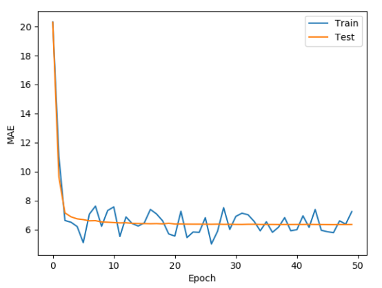
7.7 作图

plt.figure()
plt.xlabel('Epoch')
plt.ylabel('MAE')
plt.plot(train_mae_losses, label='Train')

plt.plot(test_mae_losses, label='Test')
plt.legend()

# plt.ylim([0,10])
plt.legend()
plt.savefig('auto.svg')
plt.show()