TensorFlow学习语与基本应用

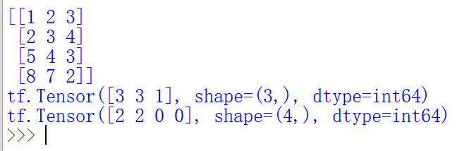
1.tensorflow中的tensor就是张量，是多维数组（多维列表），用阶来表示张量的维数，判断张量是几阶的可以看有几个方括号

例如：s = 1 2 3    0维； v =[1,2,3]     1维；   m = [[1,2,3],[4,5,6],[7,8,9]]     2维……

2.tensorflow中的数据类型：tf.int, tf.flow, …… tf.bool, tf.string……

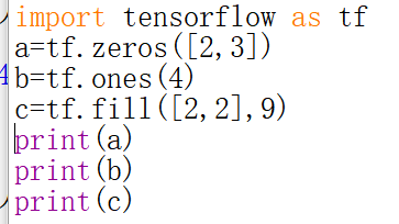
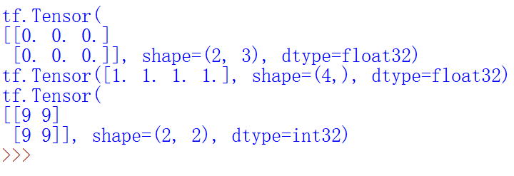
3.创建一个张量：

 

 

 

 

 

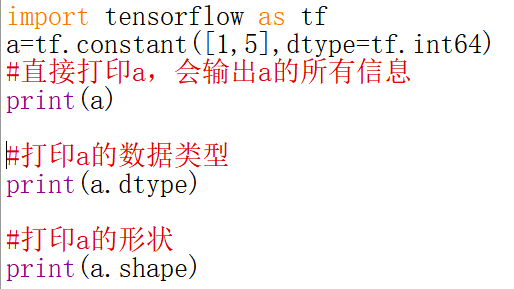
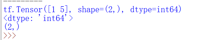
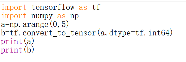
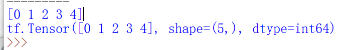
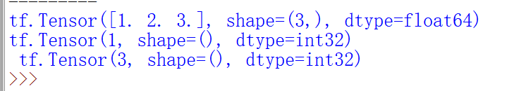
    tf.convert_to_tensor(数据名，dtype=数据类型（可选）)将numpy转化为tensor数据类型

 

 

( 

 

 

 其他方法：注意对于维度：
一维直接写个数
二维用【行，列】
多维用【m,j,k…】

 

 

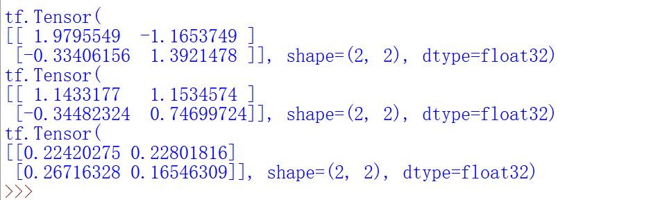
 4.生成随机数

(1)生产正态分布的随机数

(2)生成截断式正态分布的随机数

(3)生成均匀分布随机数[minval,maxval)，注意是前闭后开

 

 

 

 

 

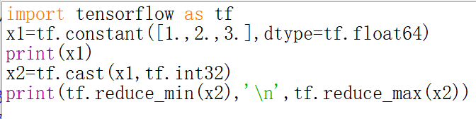
 5.常用函数

• 强制tensor转换为某数据类型 ：  tf.cast(张量名,dtype=数据类型 )

• 计算张量维度上元素的最小值 ：  tf.reduce_min(张量名)

• 计算张量维度上的元素最大值 ：  tf.reduce_max(张量名)
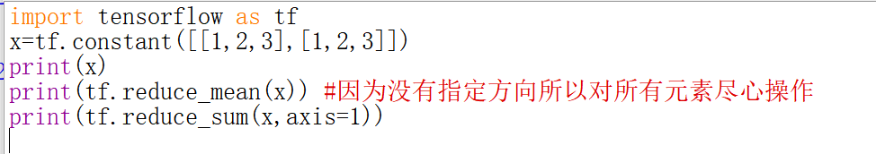
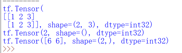
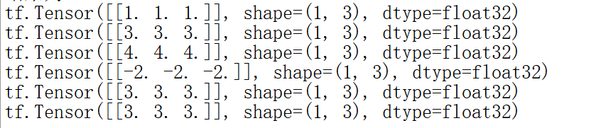
• 计算张量沿着指定方向的平均值 ：  tf.reduce_mean(张量名,axis=操作轴)
• 计算张量沿着指定维度的和 ：     tf.reduce_sum(张量名,axis=操作轴)
•   axis=0 纵向，经度方向
    axis=1 横向，维度方向

 

 

 

 

 

 

 

 

 

 

 

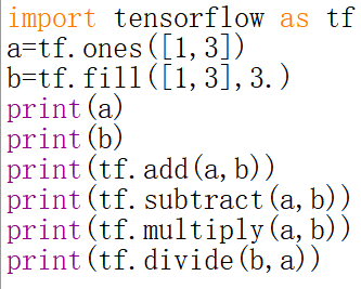
6.数学运算

  tf.add,tf.subtract,tf.multiply,tf.divide    tf.square,tf.pow,tf.sqrt（平方，次方，开方）  tf.matmul（矩阵乘法）

 

 

 

 

 

 7.数据处理

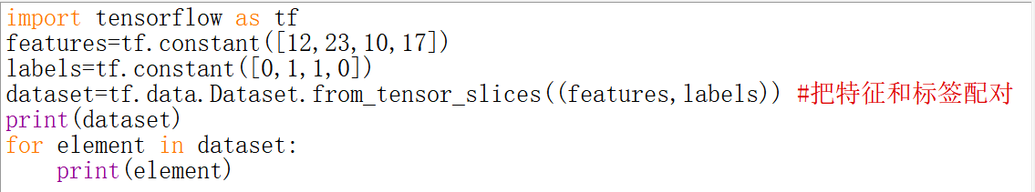
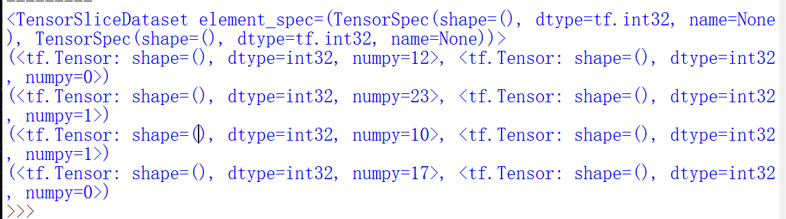
（1）from_tensor_slices切分传入张量的第一维度，生成输入标签特征/标签对，构建数据集

 

 

 

 

 

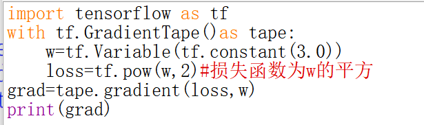
（2）tf.GradientTape实现函数求导过程

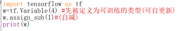
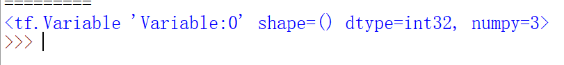
         tf.Variable()将变量标记为“可训练”tf.Variable（初始值），被标记的变量会再反向传播中记录梯度信息。神经网络训练中，常用该函数标记待训练参数

　　

 

      

 

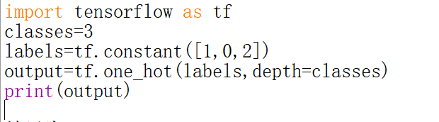
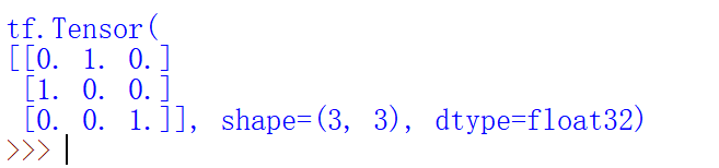
 （3）独立热编码tf.one_hot

 

 

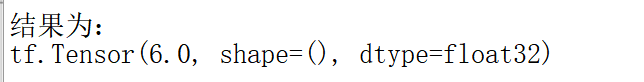
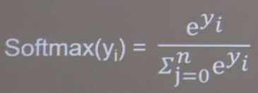
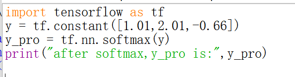
（4）通过tf.nn.softmax(x)使得输出函数符合概率分布

 

 

 

 

 

 

 

 （5）assign_sub函数 :自减操作，更新参数的值并返回

 

 

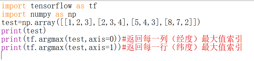
（6）tf.argmax函数，用于返回张量沿指定维度最大的索引

　　   tf.argmax(张量,axis=操作轴)

 

 

 

 

 

 

实战：

import tensorflow as tf
from tensorflow import keras
import numpy as np
import matplotlib.pyplot as plt
fashion_mnist=keras.datasets.fashion_mnist
(train_images,train_labels),(test_images,test_labels)=fashion_mnist.load_data()
class_names=['T-shirt/top','Trouser','Pullover','Dress','Coat','Sandal','Shirt','Sneaker','Bag','Ankle boot']
train_labels
train_images.shape
len(train_labels)
test_images.shape
len(test_labels)
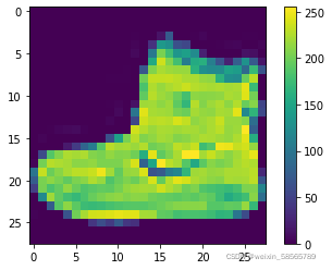
plt.figure()
plt.imshow(train_images[0])
plt.colorbar()
plt.grid(False)
plt.show()
train_images=train_images/255.0
test_images=test_images/255.0
plt.figure(figsize=(10,10))
for i in range(25):
plt.subplot(5,5,i+1)
plt.xticks([])
plt.yticks([])
plt.grid(False)
plt.imshow(train_images[i],cmap=plt.cm.binary)
plt.xlabel(class_names[train_labels[i]])
plt.show()
model=keras.Sequential([
keras.layers.Flatten(input_shape=(28,28)),
keras.layers.Dense(128,activation='relu'),
keras.layers.Dense(10)])
model.compile(optimizer='adam',
loss=tf.keras.losses.SparseCategoricalCrossentropy(from_logits=True),
metrics=['accuracy'])
model.fit(train_images,train_labels,epochs=10)
test_loss,test_acc=model.evaluate(test_images,test_labels,verbose=2)
print('\nTest accuracy:',test_acc)
probability_model=tf.keras.Sequential([model,
tf.keras.layers.Softmax()])
predictions=probability_model.predict(test_images)
predictions[0]
np.argmax(predictions[0])
test_labels[0]
def plot_image(i,predictions_array,true_label,img):
predictions_array, true_label, img=predictions_array, true_label[i], img[i]
plt.grid(False)
plt.xticks([])
plt.yticks([])
plt.imshow(img, cmap=plt.cm.binary)
predicted_label = np.argmax(predictions_array)
if predicted_label == true_label:
color = 'blue'
else:
color = 'red'

plt.xlabel("{} {:2.0f}% ({})".format(class_names[predicted_label],
100*np.max(predictions_array),
class_names[true_label]),
color=color)

def plot_value_array(i, predictions_array, true_label):
predictions_array, true_label = predictions_array, true_label[i]
plt.grid(False)
plt.xticks(range(10))
plt.yticks([])
thisplot = plt.bar(range(10), predictions_array, color="#777777")
plt.ylim([0, 1])
predicted_label = np.argmax(predictions_array)

thisplot[predicted_label].set_color('red')
thisplot[true_label].set_color('blue')
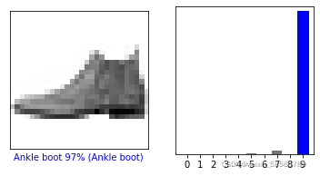
i = 0
plt.figure(figsize=(6,3))
plt.subplot(1,2,1)
plot_image(i, predictions[i], test_labels, test_images)
plt.subplot(1,2,2)
plot_value_array(i,predictions[i],test_labels)
plt.show()
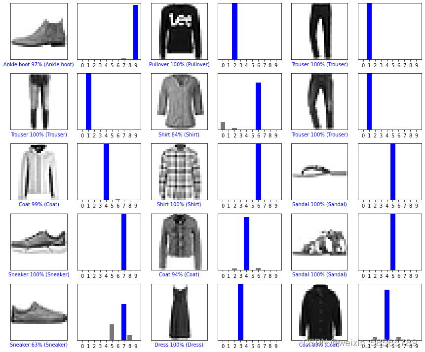
# Plot the first X test images, their predicted labels, and the true labels.
# Color correct predictions in blue and incorrect predictions in red.
num_rows = 5
num_cols = 3
num_images = num_rows*num_cols
plt.figure(figsize=(2*2*num_cols, 2*num_rows))
for i in range(num_images):
plt.subplot(num_rows,2*num_cols,2*i+1)
plot_image(i, predictions[i], test_labels, test_images)
plt.subplot(num_rows, 2*num_cols, 2*i+2)
plot_value_array(i, predictions[i], test_labels)
plt.tight_layout()
plt.show()
#测试部分
img=test_images[1]
print(img.shape)
img=(np.expand_dims(img,0))
print(img.shape)
predictions_single=probability_model.predict(img)
print(predictions_single)
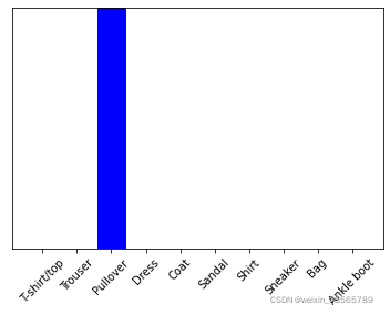
plot_value_array(1,predictions_single[0],test_labels)
_ =plt.xticks(range(10),class_names,rotation=45)
np.argmax(predictions_single[0])

结果：

 

 

 

 

 

 

 

 课后习题：

（1）

全连接 ：

层间神经元完全连接，每个输出神经元可以获取到所有输入神经元的信息，有利于信息汇总，常置于网络末层；连接与连接之间独立参数，大量的连接大大增加模型的参数规模。
局部连接：

层间神经元只有局部范围内的连接，在这个范围内采用全连接的方式，超过这个范围的神经元则没有连接；连接与连接之间独立参数，相比于全连接减少了感受域外的连接，有效减少参数规模
————————————————
版权声明：本文为CSDN博主「ys1305」的原创文章，遵循CC 4.0 BY-SA版权协议，转载请附上原文出处链接及本声明。
原文链接：https://blog.csdn.net/ys1305/article/details/99302943

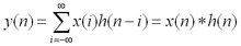
 (2)

卷积是两个变量在某范围内相乘后求和的结果。如果卷积的变量是序列x(n)和h(n)，则卷积的计算公式：

 

（3）

池化的作用：对输入的特征图进行压缩，一方面使特征图变小，简化网络计算复杂度；一方面进行特征压缩，提取主要特征。

激活函数的作用：如果不用激励函数，每一层输出都是上层输入的线性函数，无论神经网络有多少层，输出都是输入的线性组合。
如果使用的话，激活函数给神经元引入了非线性因素，使得神经网络可以任意逼近任何非线性函数，这样神经网络就可以应用到众多的非线性模型中。

（4）

局部响应归一化的作用：

1.削弱数据差异。归一化数据处理可以消除数据之间的量纲差异，便于数据利用与快速计算。

2.增强网络泛化能力。对局部神经元的活动创建竞争机制，使得其中响应比较大的值变得相对更大，并抑制其他反馈较小的神经元，增强了模型的泛化能力。LRN通过在相邻卷积核生成的feature map之间引入竞争，从而有些本来在feature map中显著的特征更显著，而在相邻的其他feature map中被抑制，这样让不同卷积核产生的feature map之间的相关性变小。
————————————————
版权声明：本文为CSDN博主「磨牙的小朋友」的原创文章，遵循CC 4.0 BY-SA版权协议，转载请附上原文出处链接及本声明。
原文链接：https://blog.csdn.net/my0npencv13poor/article/details/104510613

（5）

随机梯度下降算法的原理：

 随机梯度下降是通过每个样本来迭代更新一次，如果样本量很大的情况（例如几十万），那么可能只用其中几万条或者几千条的样本，就已经将theta迭代到最优解了，对比上面的批量梯度下降，迭代一次需要用到十几万训练样本，一次迭代不可能最优，如果迭代10次的话就需要遍历训练样本10次。但是，SGD伴随的一个问题是噪音较BGD要多，使得SGD并不是每次迭代都向着整体最优化方向。