
python爬取电竞《绝地求生》比赛数据集分析
python爬取电竞《绝地求生》比赛数据集分析
一,选题背景
电子竞技(Electronic Sports)是电子游戏比赛达到“竞技”层面的体育项目。电子竞技就是利用电子设备作为运动器械进行的、人与人之间的智力和体力结合的比拼。通过电子竞技,可以锻炼和提高参与者的思维能力、反应能力、四肢协调能力和意志力,培养团队精神,并且职业电竞对体力也有较高要求。电子竞技也是一种职业,和棋艺等非电子游戏比赛类似,2003年11月18日,国家体育局正式批准,将电子竞技列为第99个正式体育竞赛项目。2008年,国家体育总局将电子竞技改批为第78号正式体育竞赛项目。2018年雅加达亚运会将电子竞技纳为表演项目。数据来源:20G绝地求生比赛数据集。
二,设计方案
1,爬虫名称:python爬取电竞《绝地求生》比赛数据集分析
2,爬虫爬取的内容与数据特征分析
主要分成两部分,一部分是玩家比赛的统计数据,以agg_match_stats开头,一部分是玩家被击杀的数据,以kill_match_stats开头本次分析选取其中的两个数据集进行分析
3,设计方案:
-
飞机嗡嗡地,我到底跳哪里比较安全?
-
我是该苟着不动,还是应该出去猛干?
-
是该单打独斗还是跟队友一起配合?
-
毒来了我跑不过毒怎么办啊?
-
什么武器最有用?
-
近战适合使用什么武器,狙击适合使用什么武器呢?
-
最后的毒圈一般会在哪里呢?
三,结果特征分析
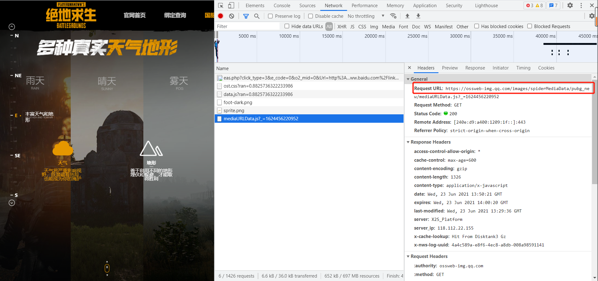
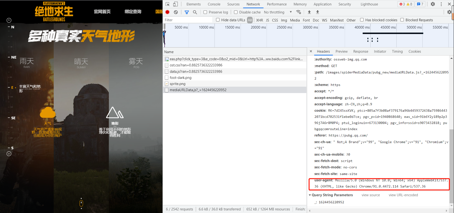
1,页面的结构与特征分析
四,程序设计
1,# 使用pandas读取数据
 1 import pandas as pd
 2 import numpy as np
 3 import matplotlib.pyplot as plt
 4 import seaborn as sns
 5 %matplotlib inline
 6 plt.rcParams['font.sans-serif'] = ['SimHei'] # 指定默认字体
 7 plt.rcParams['axes.unicode_minus'] = False # 解决保存图像是负号'-'显示为方块的问题
 8
 9 # 使用pandas读取数据
10 agg1 = pd.read_csv('/Users/apple/Desktop/pubg/aggregate/agg_match_stats_1.csv')
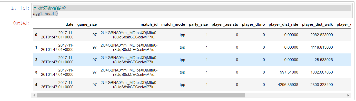
2,# 探索数据结构并数据清洗
1 agg1.head()
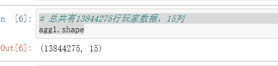
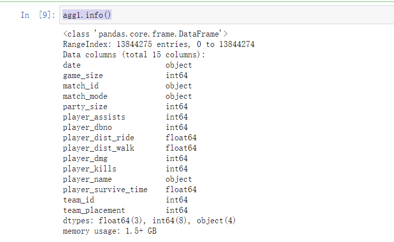
# 总共有13844275行玩家数据,15列
1 agg1.shape
1 agg1.columns

1 agg1.info()
3,数据分析与可视化
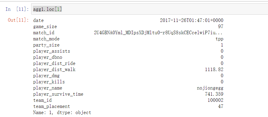
# 丢弃重复数据
1 agg1.drop_duplicates(inplace=True)
2
3 agg1.loc[1]
# 添加是否成功吃鸡列
1 agg1['won'] = agg1['team_placement'] == 1
# 添加是否搭乘过车辆列
1 agg1['drove'] = agg1['player_dist_ride'] != 0
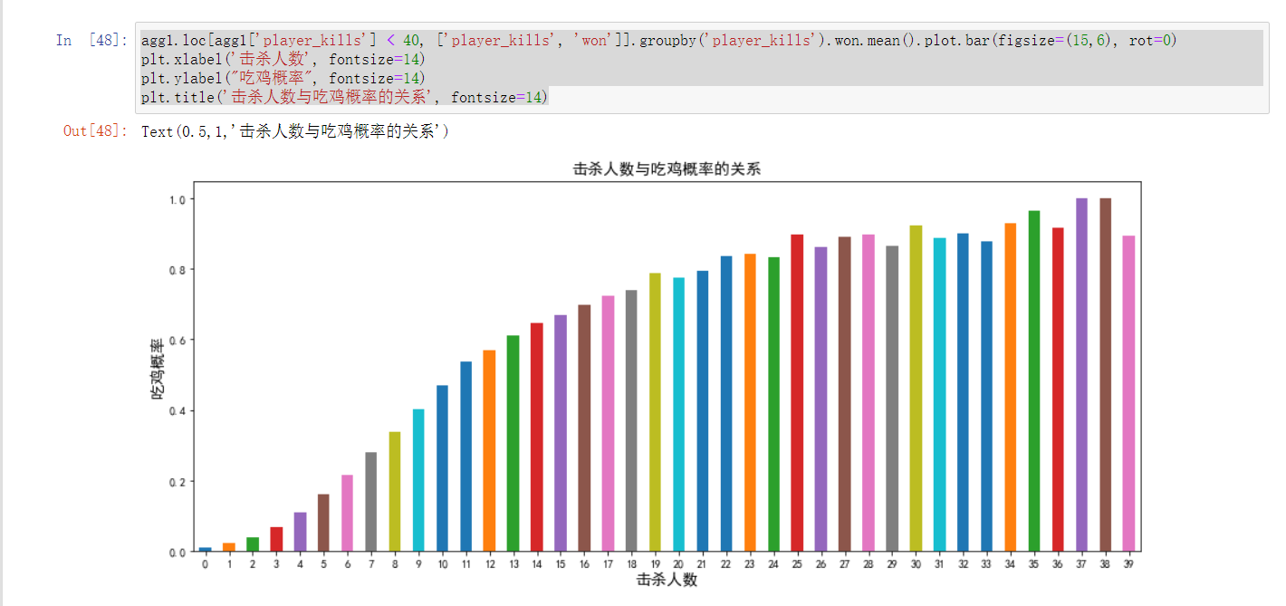
我是该苟着不动,还是应该出去猛干
1 agg1.loc[agg1['player_kills'] < 40, ['player_kills', 'won']].groupby('player_kills').won.mean().plot.bar(figsize=(15,6), rot=0)
2 plt.xlabel('击杀人数', fontsize=14)
3 plt.ylabel("吃鸡概率", fontsize=14)
4 plt.title('击杀人数与吃鸡概率的关系', fontsize=14)
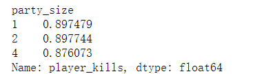
不同模式下的平均击杀人数:
1 agg1.groupby('party_size').player_kills.mean()
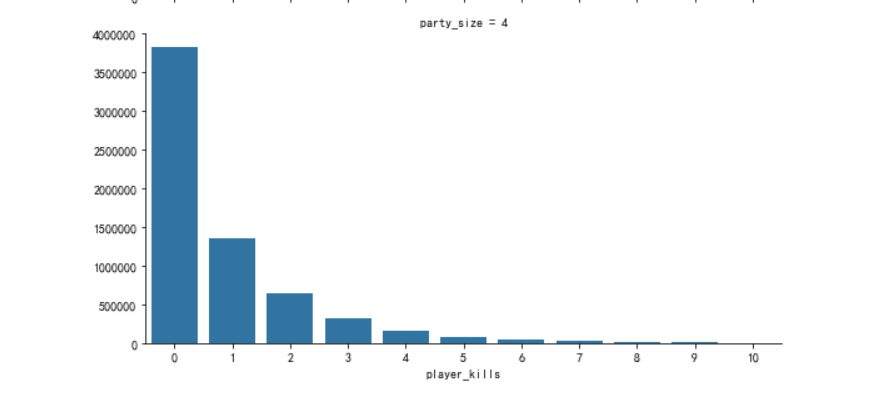
1 g = sns.FacetGrid(agg1.loc[agg1['player_kills']<=10, ['party_size', 'player_kills']], row="party_size", size=4, aspect=2)
2 g = g.map(sns.countplot, "player_kills")
3
4
5
6 party_size=1
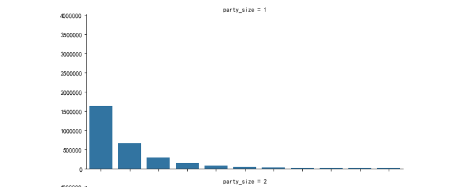
1 party_size=2
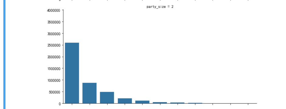
1 party_size=4
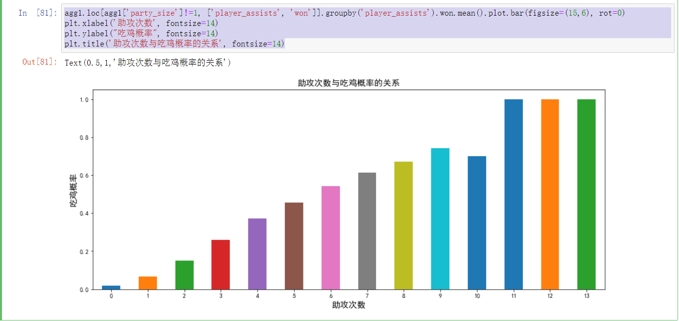
是该单打独斗还是跟队友一起配合?
1 agg1.loc[agg1['party_size']!=1, ['player_assists', 'won']].groupby('player_assists').won.mean().plot.bar(figsize=(15,6), rot=0)
2 plt.xlabel('助攻次数', fontsize=14)
3 plt.ylabel("吃鸡概率", fontsize=14)
4 plt.title('助攻次数与吃鸡概率的关系', fontsize=14)
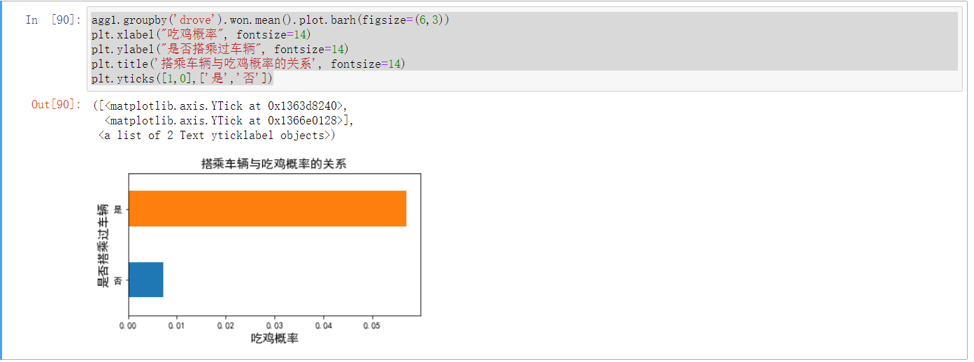
“毒来了我跑不过毒怎么办啊”之车辆到底有多重要?
1 agg1.groupby('drove').won.mean().plot.barh(figsize=(6,3))
2 plt.xlabel("吃鸡概率", fontsize=14)
3 plt.ylabel("是否搭乘过车辆", fontsize=14)
4 plt.title('搭乘车辆与吃鸡概率的关系', fontsize=14)
5 plt.yticks([1,0],['是','否'])
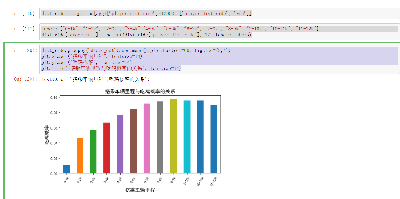
1 dist_ride = agg1.loc[agg1['player_dist_ride']<12000, ['player_dist_ride', 'won']]
2
3 labels=["0-1k", "1-2k", "2-3k", "3-4k","4-5k", "5-6k", "6-7k", "7-8k", "8-9k", "9-10k", "10-11k", "11-12k"]
4 dist_ride['drove_cut'] = pd.cut(dist_ride['player_dist_ride'], 12, labels=labels)
5
6 dist_ride.groupby('drove_cut').won.mean().plot.bar(rot=60, figsize=(8,4))
7 plt.xlabel("搭乘车辆里程", fontsize=14)
8 plt.ylabel("吃鸡概率", fontsize=14)
9 plt.title('搭乘车辆里程与吃鸡概率的关系', fontsize=14)
match_unique = agg1.loc[agg1['party_size'] == 1, 'match_id'].unique()
match_unique = agg1.loc[agg1['party_size'] == 1, 'match_id'].unique()
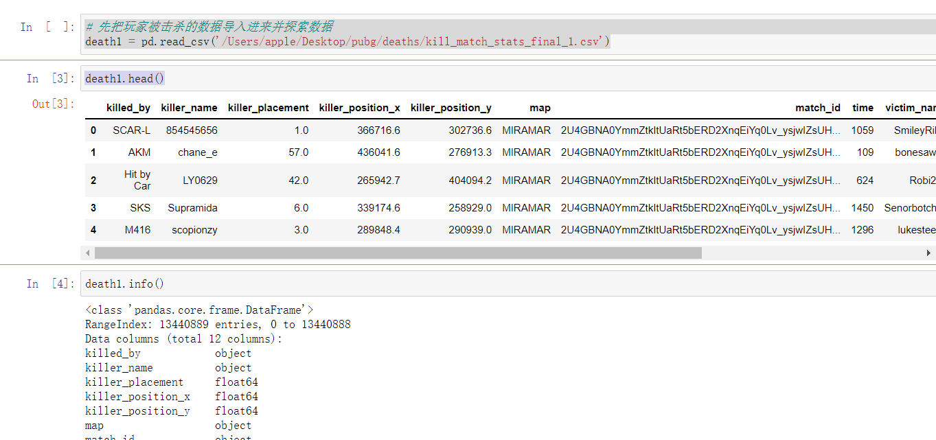
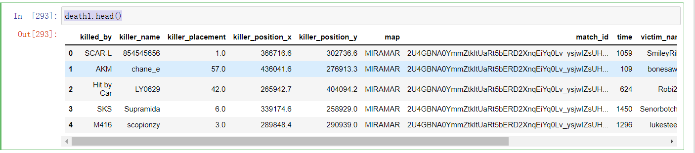
把玩家被击杀的数据导入进来
1 # 先把玩家被击杀的数据导入进来并探索数据
2 death1 = pd.read_csv('/Users/apple/Desktop/pubg/deaths/kill_match_stats_final_1.csv')
3
4 death1.head()
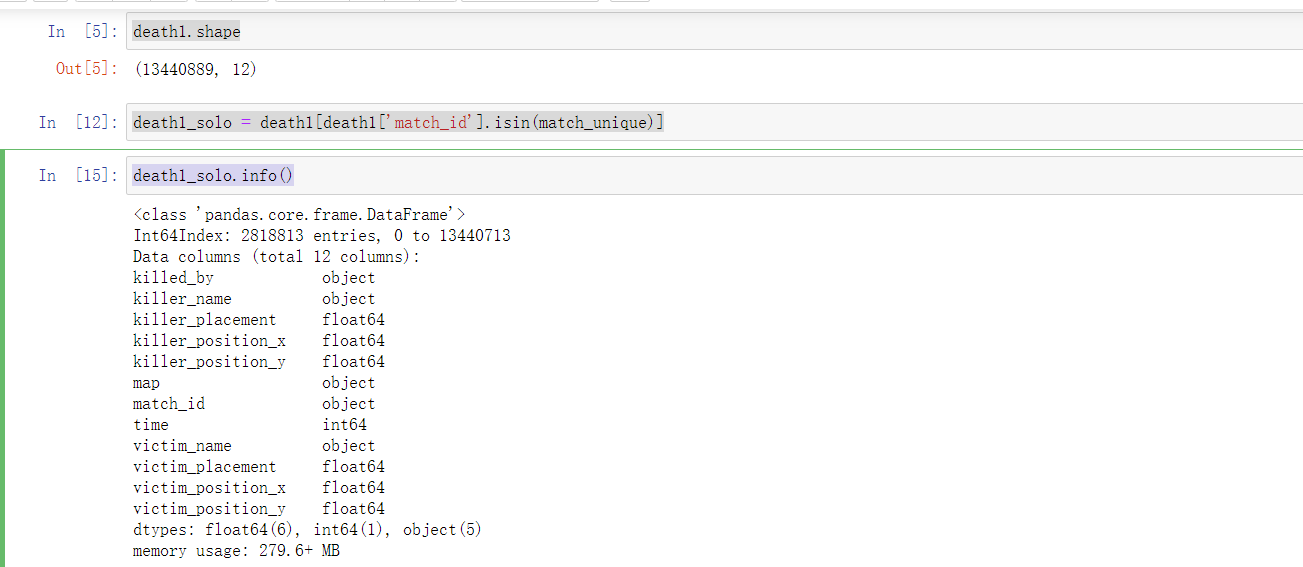
1 death1.info()
2
3 death1.shape
4
5 death1_solo = death1[death1['match_id'].isin(match_unique)]
6
7 death1_solo.info()
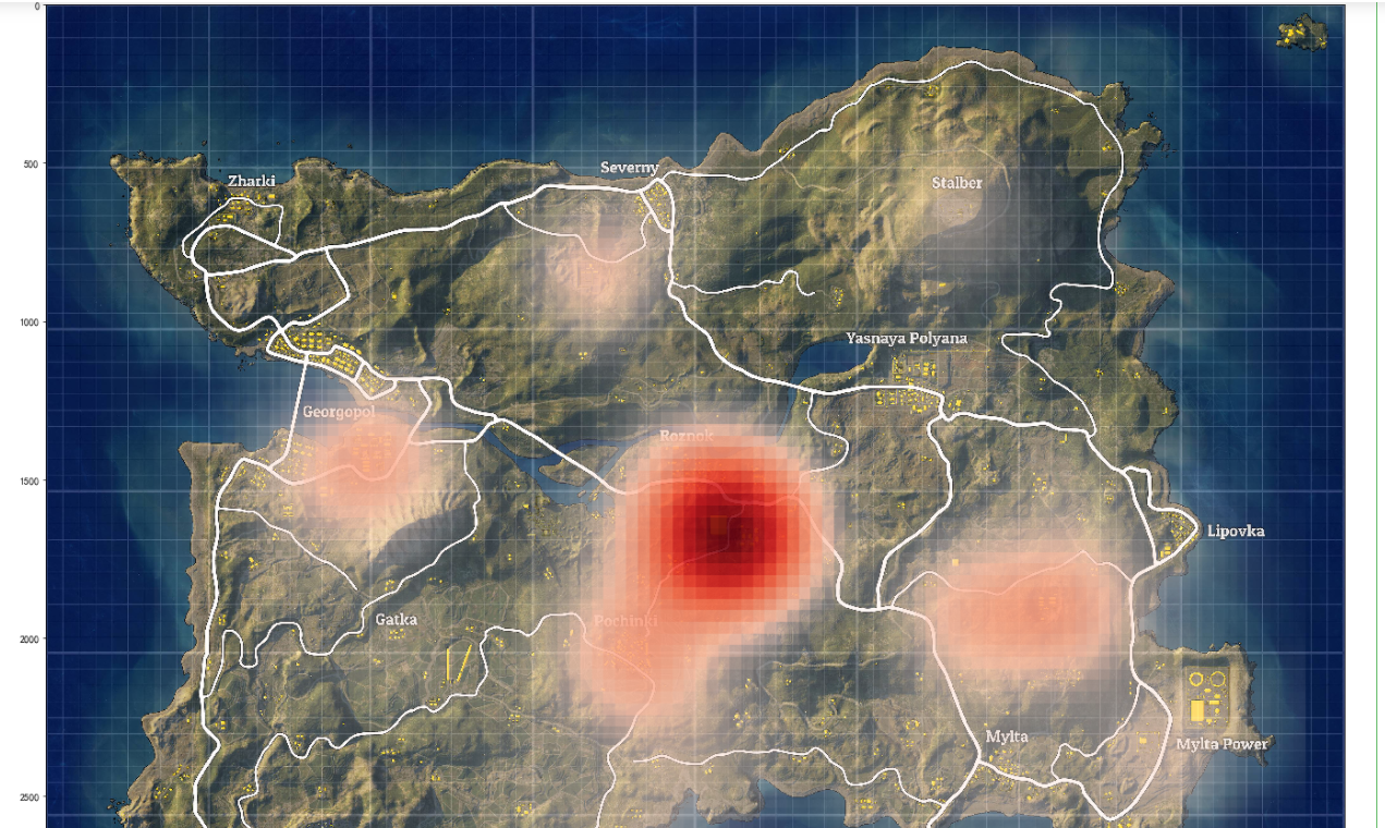
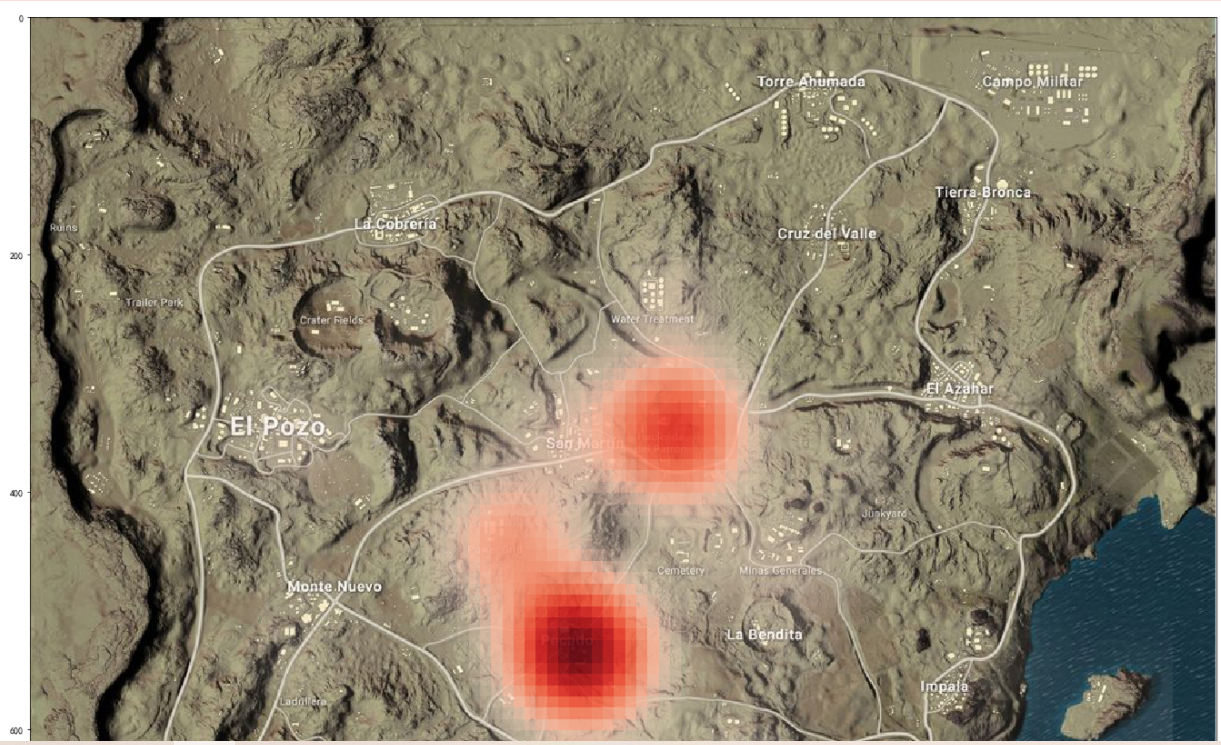
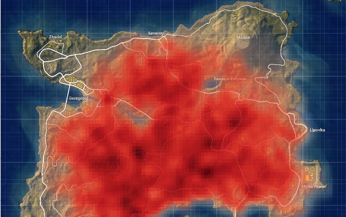
飞机嗡嗡地,我到底跳哪里比较安全
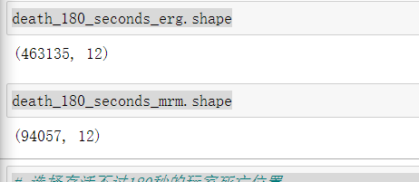
1 # 只统计单人模式,筛选存活不超过180秒的玩家数据
2 death_180_seconds_erg = death1_solo.loc[(death1_solo['map'] == 'ERANGEL')&(death1_solo['time'] < 180)&(death1_solo['victim_position_x']>0), :].dropna()
3 death_180_seconds_mrm = death1_solo.loc[(death1_solo['map'] == 'MIRAMAR')&(death1_solo['time'] < 180)&(death1_solo['victim_position_x']>0), :].dropna()
4
5 death_180_seconds_erg.shape
6
7 death_180_seconds_mrm.shape
 1 # 选择存活不过180秒的玩家死亡位置
 2 data_erg = death_180_seconds_erg[['victim_position_x', 'victim_position_y']].values
 3 data_mrm = death_180_seconds_mrm[['victim_position_x', 'victim_position_y']].values
 4
 5 # 重新scale玩家位置
 6 data_erg = data_erg*4096/800000
 7 data_mrm = data_mrm*1000/800000
 8
 9 from scipy.ndimage.filters import gaussian_filter
10 import matplotlib.cm as cm
11 from matplotlib.colors import Normalize
12 from scipy.misc.pilutil import imread
13
14 from scipy.ndimage.filters import gaussian_filter
15 import matplotlib.cm as cm
16 from matplotlib.colors import Normalize
17
18 def heatmap(x, y, s, bins=100):
19 heatmap, xedges, yedges = np.histogram2d(x, y, bins=bins)
20 heatmap = gaussian_filter(heatmap, sigma=s)
21
22 extent = [xedges[0], xedges[-1], yedges[0], yedges[-1]]
23 return heatmap.T, extent
24
25 bg = imread('/Users/apple/Desktop/pubg/erangel.jpg')
26 hmap, extent = heatmap(data_erg[:,0], data_erg[:,1], 4.5)
27 alphas = np.clip(Normalize(0, hmap.max(), clip=True)(hmap)*4.5, 0.0, 1.)
28 colors = Normalize(0, hmap.max(), clip=True)(hmap)
29 colors = cm.Reds(colors)
30 colors[..., -1] = alphas
31
32 fig, ax = plt.subplots(figsize=(24,24))
33 ax.set_xlim(0, 4096); ax.set_ylim(0, 4096)
34 ax.imshow(bg)
35 ax.imshow(colors, extent=extent, origin='lower', cmap=cm.Reds, alpha=0.9)
36 plt.gca().invert_yaxis()
 1 bg = imread('/Users/apple/Desktop/pubg/miramar.jpg')
 2 hmap, extent = heatmap(data_mrm[:,0], data_mrm[:,1], 4)
 3 alphas = np.clip(Normalize(0, hmap.max(), clip=True)(hmap)*4, 0.0, 1.)
 4 colors = Normalize(0, hmap.max(), clip=True)(hmap)
 5 colors = cm.Reds(colors)
 6 colors[..., -1] = alphas
 7
 8 fig, ax = plt.subplots(figsize=(24,24))
 9 ax.set_xlim(0, 1000); ax.set_ylim(0, 1000)
10 ax.imshow(bg)
11 ax.imshow(colors, extent=extent, origin='lower', cmap=cm.Reds, alpha=0.9)
12 #plt.scatter(plot_data_mr[:,0], plot_data_mr[:,1])
13 plt.gca().invert_yaxis()
最后的毒圈一般会在哪里呢?
这里选取每场比赛第一名和第二名的位置数据,因为第一名和第二名所在的位置基本上就是最后的毒圈所在的位置
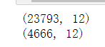
 1 death_final_circle_erg = death1_solo.loc[(death1_solo['map'] == 'ERANGEL')&(death1_solo['victim_placement'] == 2)&(death1_solo['victim_position_x']>0)&(death1_solo['killer_position_x']>0), :].dropna()
 2 death_final_circle_mrm = death1_solo.loc[(death1_solo['map'] == 'MIRAMAR')&(death1_solo['victim_placement'] == 2)&(death1_solo['victim_position_x']>0)&(death1_solo['killer_position_x']>0), :].dropna()
 3
 4 print(death_final_circle_erg.shape)
 5 print(death_final_circle_mrm.shape)
 6
 7 final_circle_erg = np.vstack([death_final_circle_erg[['victim_position_x', 'victim_position_y']].values,
 8 death_final_circle_erg[['killer_position_x', 'killer_position_y']].values])*4096/800000
 9 final_circle_mrm = np.vstack([death_final_circle_mrm[['victim_position_x', 'victim_position_y']].values,
10 death_final_circle_mrm[['killer_position_x', 'killer_position_y']].values])*1000/800000
 1 bg = imread('/Users/apple/Desktop/pubg/erangel.jpg')
 2 hmap, extent = heatmap(final_circle_erg[:,0], final_circle_erg[:,1], 1.5)
 3 alphas = np.clip(Normalize(0, hmap.max(), clip=True)(hmap)*1.5, 0.0, 1.)
 4 colors = Normalize(0, hmap.max(), clip=True)(hmap)
 5 colors = cm.Reds(colors)
 6 colors[..., -1] = alphas
 7
 8 fig, ax = plt.subplots(figsize=(24,24))
 9 ax.set_xlim(0, 4096); ax.set_ylim(0, 4096)
10 ax.imshow(bg)
11 ax.imshow(colors, extent=extent, origin='lower', cmap=cm.Reds, alpha=0.9)
12 #plt.scatter(plot_data_er[:,0], plot_data_er[:,1])
13
14 plt.gca().invert_yaxis()
 1 bg = imread('/Users/apple/Desktop/pubg/miramar.jpg')
 2 hmap, extent = heatmap(final_circle_mrm[:,0], final_circle_mrm[:,1], 1.5)
 3 alphas = np.clip(Normalize(0, hmap.max(), clip=True)(hmap)*1.5, 0.0, 1.)
 4 colors = Normalize(0, hmap.max(), clip=True)(hmap)
 5 colors = cm.Reds(colors)
 6 colors[..., -1] = alphas
 7
 8 fig, ax = plt.subplots(figsize=(24,24))
 9 ax.set_xlim(0, 1000); ax.set_ylim(0, 1000)
10 ax.imshow(bg)
11 ax.imshow(colors, extent=extent, origin='lower', cmap=cm.Reds, alpha=0.9)
12 #plt.scatter(plot_data_mr[:,0], plot_data_mr[:,1])
13 plt.gca().invert_yaxis()

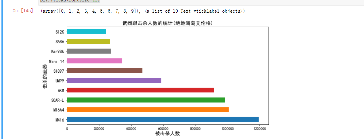
什么武器最有用?
1 erg_died_of = death1.loc[(death1['map']=='ERANGEL')&(death1['killer_position_x']>0)&(death1['victim_position_x']>0)&(death1['killed_by']!='Down and Out'),:]
2 mrm_died_of = death1.loc[(death1['map']=='MIRAMAR')&(death1['killer_position_x']>0)&(death1['victim_position_x']>0)&(death1['killed_by']!='Down and Out'),:]
3
4 print(erg_died_of.shape)
5 print(mrm_died_of.shape)

1 erg_died_of['killed_by'].value_counts()[:10].plot.barh(figsize=(10,5))
2 plt.xlabel("被击杀人数", fontsize=14)
3 plt.ylabel("击杀的武器", fontsize=14)
4 plt.title('武器跟击杀人数的统计(绝地海岛艾伦格)', fontsize=14)
5 plt.yticks(fontsize=12)
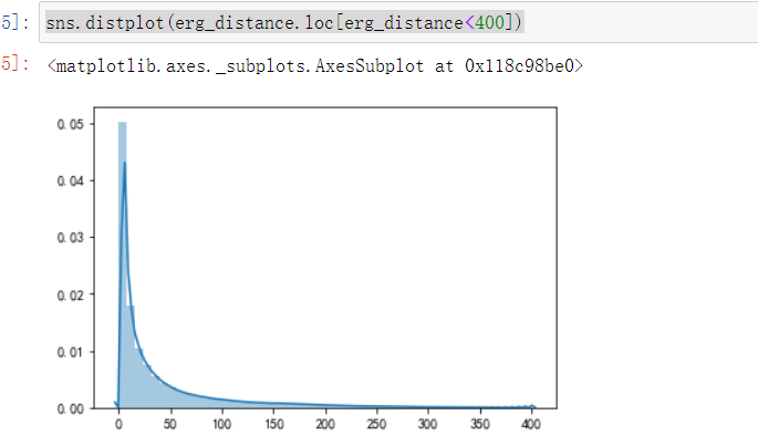
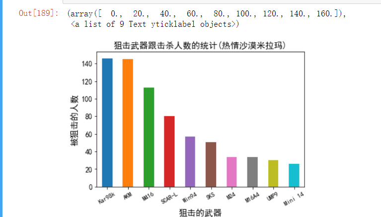
狙击适合使用什么武器?
 1 # 把位置信息转换成距离,以“米”为单位
 2 erg_distance = np.sqrt(((erg_died_of['killer_position_x']-erg_died_of['victim_position_x'])/100)**2 + ((erg_died_of['killer_position_y']-erg_died_of['victim_position_y'])/100)**2)
 3
 4
 5
 6 mrm_distance = np.sqrt(((mrm_died_of['killer_position_x']-mrm_died_of['victim_position_x'])/100)**2 + ((mrm_died_of['killer_position_y']-mrm_died_of['victim_position_y'])/100)**2)
 7
 8
 9
10 sns.distplot(erg_distance.loc[erg_distance<400])
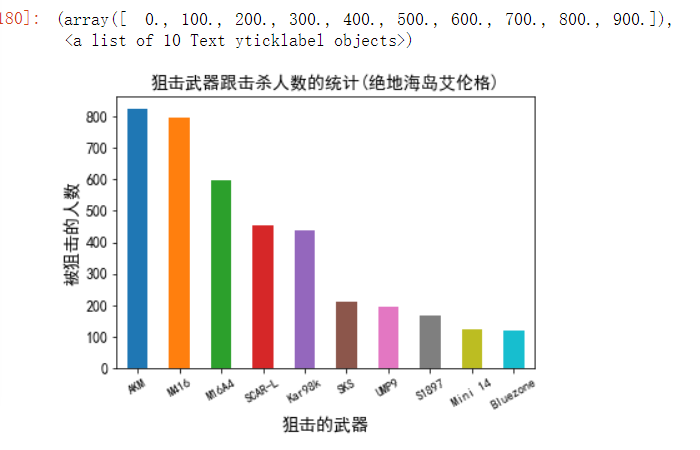
1 erg_died_of.loc[(erg_distance > 800)&(erg_distance < 1500), 'killed_by'].value_counts()[:10].plot.bar(rot=30)
2 plt.xlabel("狙击的武器", fontsize=14)
3 plt.ylabel("被狙击的人数", fontsize=14)
4 plt.title('狙击武器跟击杀人数的统计(绝地海岛艾伦格)', fontsize=14)
5 plt.yticks(fontsize=12)
1 mrm_died_of.loc[(mrm_distance > 800)&(mrm_distance < 1000), 'killed_by'].value_counts()[:10].plot.bar(rot=30)
2 plt.xlabel("狙击的武器", fontsize=14)
3 plt.ylabel("被狙击的人数", fontsize=14)
4 plt.title('狙击武器跟击杀人数的统计(热情沙漠米拉玛)', fontsize=14)
5 plt.yticks(fontsize=12)
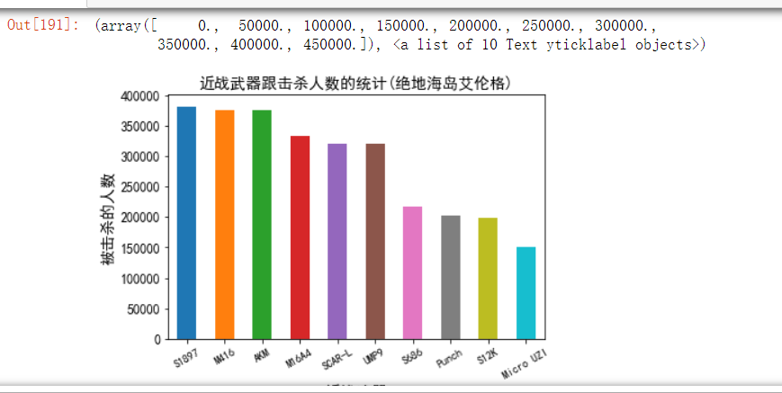
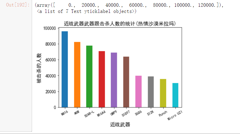
近战适合使用什么武器?
1 erg_died_of.loc[erg_distance<10, 'killed_by'].value_counts()[:10].plot.bar(rot=30)
2 plt.xlabel("近战武器", fontsize=14)
3 plt.ylabel("被击杀的人数", fontsize=14)
4 plt.title('近战武器跟击杀人数的统计(绝地海岛艾伦格)', fontsize=14)
5 plt.yticks(fontsize=12)
1 mrm_died_of.loc[mrm_distance<10, 'killed_by'].value_counts()[:10].plot.bar(rot=30)
2 plt.xlabel("近战武器", fontsize=14)
3 plt.ylabel("被击杀的人数", fontsize=14)
4 plt.title('近战武器武器跟击杀人数的统计(热情沙漠米拉玛)', fontsize=14)
5 plt.yticks(fontsize=12)
Top10武器在各距离下的击杀百分比
  1 erg_died_of['erg_dist'] = erg_distance
  2 erg_died_of = erg_died_of.loc[erg_died_of['erg_dist']<800, :]
  3 top_weapons_erg = list(erg_died_of['killed_by'].value_counts()[:10].index)
  4 top_weapon_kills = erg_died_of[np.in1d(erg_died_of['killed_by'], top_weapons_erg)].copy()
  5 top_weapon_kills['bin'] = pd.cut(top_weapon_kills['erg_dist'], np.arange(0, 800, 10), include_lowest=True, labels=False)
  6 top_weapon_kills_wide = top_weapon_kills.groupby(['killed_by', 'bin']).size().unstack(fill_value=0).transpose()
  7
  8
  9
 10 top_weapon_kills_wide = top_weapon_kills_wide.div(top_weapon_kills_wide.sum(axis=1), axis=0)
 11
 12
 13
 14 from bokeh.models.tools import HoverTool
 15 from bokeh.palettes import brewer
 16 from bokeh.plotting import figure, show, output_notebook
 17 from bokeh.models.sources import ColumnDataSource
 18
 19 def stacked(df):
 20 df_top = df.cumsum(axis=1)
 21 df_bottom = df_top.shift(axis=1).fillna(0)[::-1]
 22 df_stack = pd.concat([df_bottom, df_top], ignore_index=True)
 23 return df_stack
 24
 25 hover = HoverTool(
 26 tooltips=[
 27 ("index", "$index"),
 28 ("weapon", "@weapon"),
 29 ("(x,y)", "($x, $y)")
 30 ],
 31 point_policy='follow_mouse'
 32 )
 33
 34 areas = stacked(top_weapon_kills_wide)
 35
 36 colors = brewer['Spectral'][areas.shape[1]]
 37 x2 = np.hstack((top_weapon_kills_wide.index[::-1],
 38 top_weapon_kills_wide.index)) /0.095
 39
 40 TOOLS="pan,wheel_zoom,box_zoom,reset,previewsave"
 41 output_notebook()
 42 p = figure(x_range=(1, 800), y_range=(0, 1), tools=[TOOLS, hover], plot_width=800)
 43 p.grid.minor_grid_line_color = '#eeeeee'
 44
 45 source = ColumnDataSource(data={
 46 'x': [x2] * areas.shape[1],
 47 'y': [areas[c].values for c in areas],
 48 'weapon': list(top_weapon_kills_wide.columns),
 49 'color': colors
 50 })
 51
 52 p.patches('x', 'y', source=source, legend="weapon",
 53 color='color', alpha=0.8, line_color=None)
 54 p.title.text = "Top10武器在各距离下的击杀百分比(绝地海岛艾伦格)"
 55 p.xaxis.axis_label = "击杀距离(0-800米)"
 56 p.yaxis.axis_label = "百分比"
 57
 58 show(p)
 59
 60
 61
 62 mrm_died_of['erg_dist'] = mrm_distance
 63 mrm_died_of = mrm_died_of.loc[mrm_died_of['erg_dist']<800, :]
 64 top_weapons_erg = list(mrm_died_of['killed_by'].value_counts()[:10].index)
 65 top_weapon_kills = mrm_died_of[np.in1d(mrm_died_of['killed_by'], top_weapons_erg)].copy()
 66 top_weapon_kills['bin'] = pd.cut(top_weapon_kills['erg_dist'], np.arange(0, 800, 10), include_lowest=True, labels=False)
 67 top_weapon_kills_wide = top_weapon_kills.groupby(['killed_by', 'bin']).size().unstack(fill_value=0).transpose()
 68
 69 top_weapon_kills_wide = top_weapon_kills_wide.div(top_weapon_kills_wide.sum(axis=1), axis=0)
 70
 71
 72
 73 def stacked(df):
 74 df_top = df.cumsum(axis=1)
 75 df_bottom = df_top.shift(axis=1).fillna(0)[::-1]
 76 df_stack = pd.concat([df_bottom, df_top], ignore_index=True)
 77 return df_stack
 78
 79 hover = HoverTool(
 80 tooltips=[
 81 ("index", "$index"),
 82 ("weapon", "@weapon"),
 83 ("(x,y)", "($x, $y)")
 84 ],
 85 point_policy='follow_mouse'
 86 )
 87
 88 areas = stacked(top_weapon_kills_wide)
 89
 90 colors = brewer['Spectral'][areas.shape[1]]
 91 x2 = np.hstack((top_weapon_kills_wide.index[::-1],
 92 top_weapon_kills_wide.index)) /0.095
 93
 94 TOOLS="pan,wheel_zoom,box_zoom,reset,previewsave"
 95 output_notebook()
 96 p = figure(x_range=(1, 800), y_range=(0, 1), tools=[TOOLS, hover], plot_width=800)
 97 p.grid.minor_grid_line_color = '#eeeeee'
 98
 99 source = ColumnDataSource(data={
100 'x': [x2] * areas.shape[1],
101 'y': [areas[c].values for c in areas],
102 'weapon': list(top_weapon_kills_wide.columns),
103 'color': colors
104 })
105
106 p.patches('x', 'y', source=source, legend="weapon",
107 color='color', alpha=0.8, line_color=None)
108 p.title.text = "Top10武器在各距离下的击杀百分比(热情沙漠米拉玛)"
109 p.xaxis.axis_label = "击杀距离(0-800米)"
110 p.yaxis.axis_label = "击杀百分比"
111
112 show(p)
自己把自己干倒的方式与人数
1 death1.head()
1  kill_by_self = death1.loc[death1['killer_name']==death1['victim_name'], "killed_by"]
2
3 kill_by_self.value_counts()[:10].plot.barh()
4 plt.xlabel("自毙的人数", fontsize=14)
5 plt.ylabel("自毙的方式", fontsize=14)
6 plt.title('自己把自己干倒的方式与人数', fontsize=14)
7 plt.yticks(fontsize=12)
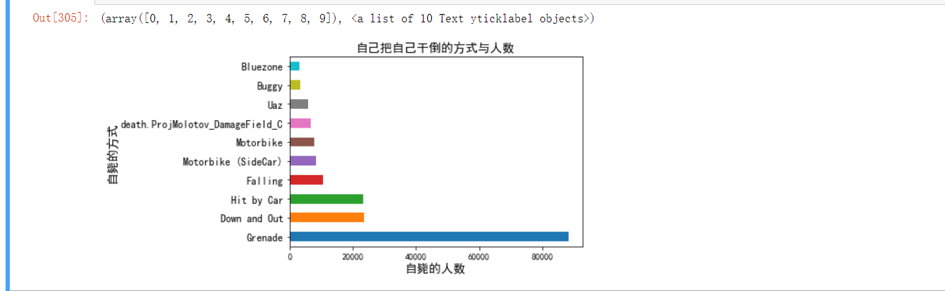
1 # 自己把自己干倒的人数场均百分比
2 kill_by_self.shape[0]/death1.shape[0]*100
完整代码:
  1 import pandas as pd
  2 import numpy as np
  3 import matplotlib.pyplot as plt
  4 import seaborn as sns
  5 %matplotlib inline
  6 plt.rcParams['font.sans-serif'] = ['SimHei'] # 指定默认字体
  7 plt.rcParams['axes.unicode_minus'] = False # 解决保存图像是负号'-'显示为方块的问题
  8
  9 # 使用pandas读取数据
 10 agg1 = pd.read_csv('/Users/apple/Desktop/pubg/aggregate/agg_match_stats_1.csv')
 11
 12 # 探索数据结构
 13 agg1.head()
 14
 15 # 总共有13844275行玩家数据,15列
 16 agg1.shape
 17
 18 agg1.columns
 19
 20 agg1.info()
 21
 22 # 丢弃重复数据
 23 agg1.drop_duplicates(inplace=True)
 24
 25 agg1.loc[1]
 26
 27 # 添加是否成功吃鸡列
 28 agg1['won'] = agg1['team_placement'] == 1
 29
 30 # 添加是否搭乘过车辆列
 31 agg1['drove'] = agg1['player_dist_ride'] != 0
 32
 33 agg1.loc[agg1['player_kills'] < 40, ['player_kills', 'won']].groupby('player_kills').won.mean().plot.bar(figsize=(15,6), rot=0)
 34 plt.xlabel('击杀人数', fontsize=14)
 35 plt.ylabel("吃鸡概率", fontsize=14)
 36 plt.title('击杀人数与吃鸡概率的关系', fontsize=14)
 37
 38 agg1.groupby('party_size').player_kills.mean()
 39
 40 g = sns.FacetGrid(agg1.loc[agg1['player_kills']<=10, ['party_size', 'player_kills']], row="party_size", size=4, aspect=2)
 41 g = g.map(sns.countplot, "player_kills")
 42
 43 agg1.loc[agg1['party_size']!=1, ['player_assists', 'won']].groupby('player_assists').won.mean().plot.bar(figsize=(15,6), rot=0)
 44 plt.xlabel('助攻次数', fontsize=14)
 45 plt.ylabel("吃鸡概率", fontsize=14)
 46 plt.title('助攻次数与吃鸡概率的关系', fontsize=14)
 47
 48 agg1.groupby('drove').won.mean().plot.barh(figsize=(6,3))
 49 plt.xlabel("吃鸡概率", fontsize=14)
 50 plt.ylabel("是否搭乘过车辆", fontsize=14)
 51 plt.title('搭乘车辆与吃鸡概率的关系', fontsize=14)
 52 plt.yticks([1,0],['是','否'])
 53
 54 dist_ride = agg1.loc[agg1['player_dist_ride']<12000, ['player_dist_ride', 'won']]
 55
 56 labels=["0-1k", "1-2k", "2-3k", "3-4k","4-5k", "5-6k", "6-7k", "7-8k", "8-9k", "9-10k", "10-11k", "11-12k"]
 57 dist_ride['drove_cut'] = pd.cut(dist_ride['player_dist_ride'], 12, labels=labels)
 58
 59 dist_ride.groupby('drove_cut').won.mean().plot.bar(rot=60, figsize=(8,4))
 60 plt.xlabel("搭乘车辆里程", fontsize=14)
 61 plt.ylabel("吃鸡概率", fontsize=14)
 62 plt.title('搭乘车辆里程与吃鸡概率的关系', fontsize=14)
 63
 64 match_unique = agg1.loc[agg1['party_size'] == 1, 'match_id'].unique()
 65
 66 # 先把玩家被击杀的数据导入进来并探索数据
 67 death1 = pd.read_csv('/Users/apple/Desktop/pubg/deaths/kill_match_stats_final_1.csv')
 68
 69 death1.head()
 70
 71 death1.info()
 72
 73 death1.shape
 74
 75 death1_solo = death1[death1['match_id'].isin(match_unique)]
 76
 77 death1_solo.info()
 78
 79 # 只统计单人模式,筛选存活不超过180秒的玩家数据
 80 death_180_seconds_erg = death1_solo.loc[(death1_solo['map'] == 'ERANGEL')&(death1_solo['time'] < 180)&(death1_solo['victim_position_x']>0), :].dropna()
 81 death_180_seconds_mrm = death1_solo.loc[(death1_solo['map'] == 'MIRAMAR')&(death1_solo['time'] < 180)&(death1_solo['victim_position_x']>0), :].dropna()
 82
 83 death_180_seconds_erg.shape
 84
 85 death_180_seconds_mrm.shape
 86
 87 # 选择存活不过180秒的玩家死亡位置
 88 data_erg = death_180_seconds_erg[['victim_position_x', 'victim_position_y']].values
 89 data_mrm = death_180_seconds_mrm[['victim_position_x', 'victim_position_y']].values
 90
 91 # 重新scale玩家位置
 92 data_erg = data_erg*4096/800000
 93 data_mrm = data_mrm*1000/800000
 94
 95 from scipy.ndimage.filters import gaussian_filter
 96 import matplotlib.cm as cm
 97 from matplotlib.colors import Normalize
 98 from scipy.misc.pilutil import imread
 99
100 from scipy.ndimage.filters import gaussian_filter
101 import matplotlib.cm as cm
102 from matplotlib.colors import Normalize
103
104 def heatmap(x, y, s, bins=100):
105     heatmap, xedges, yedges = np.histogram2d(x, y, bins=bins)
106     heatmap = gaussian_filter(heatmap, sigma=s)
107
108     extent = [xedges[0], xedges[-1], yedges[0], yedges[-1]]
109     return heatmap.T, extent
110
111 bg = imread('/Users/apple/Desktop/pubg/erangel.jpg')
112 hmap, extent = heatmap(data_erg[:,0], data_erg[:,1], 4.5)
113 alphas = np.clip(Normalize(0, hmap.max(), clip=True)(hmap)*4.5, 0.0, 1.)
114 colors = Normalize(0, hmap.max(), clip=True)(hmap)
115 colors = cm.Reds(colors)
116 colors[..., -1] = alphas
117
118 fig, ax = plt.subplots(figsize=(24,24))
119 ax.set_xlim(0, 4096); ax.set_ylim(0, 4096)
120 ax.imshow(bg)
121 ax.imshow(colors, extent=extent, origin='lower', cmap=cm.Reds, alpha=0.9)
122 plt.gca().invert_yaxis()
123
124 bg = imread('/Users/apple/Desktop/pubg/miramar.jpg')
125 hmap, extent = heatmap(data_mrm[:,0], data_mrm[:,1], 4)
126 alphas = np.clip(Normalize(0, hmap.max(), clip=True)(hmap)*4, 0.0, 1.)
127 colors = Normalize(0, hmap.max(), clip=True)(hmap)
128 colors = cm.Reds(colors)
129 colors[..., -1] = alphas
130
131 fig, ax = plt.subplots(figsize=(24,24))
132 ax.set_xlim(0, 1000); ax.set_ylim(0, 1000)
133 ax.imshow(bg)
134 ax.imshow(colors, extent=extent, origin='lower', cmap=cm.Reds, alpha=0.9)
135 #plt.scatter(plot_data_mr[:,0], plot_data_mr[:,1])
136 plt.gca().invert_yaxis()
137
138 death_final_circle_erg = death1_solo.loc[(death1_solo['map'] == 'ERANGEL')&(death1_solo['victim_placement'] == 2)&(death1_solo['victim_position_x']>0)&(death1_solo['killer_position_x']>0), :].dropna()
139 death_final_circle_mrm = death1_solo.loc[(death1_solo['map'] == 'MIRAMAR')&(death1_solo['victim_placement'] == 2)&(death1_solo['victim_position_x']>0)&(death1_solo['killer_position_x']>0), :].dropna()
140
141 print(death_final_circle_erg.shape)
142 print(death_final_circle_mrm.shape)
143
144 final_circle_erg = np.vstack([death_final_circle_erg[['victim_position_x', 'victim_position_y']].values,
145                                     death_final_circle_erg[['killer_position_x', 'killer_position_y']].values])*4096/800000
146 final_circle_mrm = np.vstack([death_final_circle_mrm[['victim_position_x', 'victim_position_y']].values,
147                                     death_final_circle_mrm[['killer_position_x', 'killer_position_y']].values])*1000/800000
148
149 bg = imread('/Users/apple/Desktop/pubg/erangel.jpg')
150 hmap, extent = heatmap(final_circle_erg[:,0], final_circle_erg[:,1], 1.5)
151 alphas = np.clip(Normalize(0, hmap.max(), clip=True)(hmap)*1.5, 0.0, 1.)
152 colors = Normalize(0, hmap.max(), clip=True)(hmap)
153 colors = cm.Reds(colors)
154 colors[..., -1] = alphas
155
156 fig, ax = plt.subplots(figsize=(24,24))
157 ax.set_xlim(0, 4096); ax.set_ylim(0, 4096)
158 ax.imshow(bg)
159 ax.imshow(colors, extent=extent, origin='lower', cmap=cm.Reds, alpha=0.9)
160 #plt.scatter(plot_data_er[:,0], plot_data_er[:,1])
161 plt.gca().invert_yaxis()
162
163 bg = imread('/Users/apple/Desktop/pubg/miramar.jpg')
164 hmap, extent = heatmap(final_circle_mrm[:,0], final_circle_mrm[:,1], 1.5)
165 alphas = np.clip(Normalize(0, hmap.max(), clip=True)(hmap)*1.5, 0.0, 1.)
166 colors = Normalize(0, hmap.max(), clip=True)(hmap)
167 colors = cm.Reds(colors)
168 colors[..., -1] = alphas
169
170 fig, ax = plt.subplots(figsize=(24,24))
171 ax.set_xlim(0, 1000); ax.set_ylim(0, 1000)
172 ax.imshow(bg)
173 ax.imshow(colors, extent=extent, origin='lower', cmap=cm.Reds, alpha=0.9)
174 #plt.scatter(plot_data_mr[:,0], plot_data_mr[:,1])
175 plt.gca().invert_yaxis()
176
177 erg_died_of = death1.loc[(death1['map']=='ERANGEL')&(death1['killer_position_x']>0)&(death1['victim_position_x']>0)&(death1['killed_by']!='Down and Out'),:]
178 mrm_died_of = death1.loc[(death1['map']=='MIRAMAR')&(death1['killer_position_x']>0)&(death1['victim_position_x']>0)&(death1['killed_by']!='Down and Out'),:]
179
180 print(erg_died_of.shape)
181 print(mrm_died_of.shape)
182
183 erg_died_of['killed_by'].value_counts()[:10].plot.barh(figsize=(10,5))
184 plt.xlabel("被击杀人数", fontsize=14)
185 plt.ylabel("击杀的武器", fontsize=14)
186 plt.title('武器跟击杀人数的统计(绝地海岛艾伦格)', fontsize=14)
187 plt.yticks(fontsize=12)
188
189 mrm_died_of['killed_by'].value_counts()[:10].plot.barh(figsize=(10,5))
190 plt.xlabel("被击杀人数", fontsize=14)
191 plt.ylabel("击杀的武器", fontsize=14)
192 plt.title('武器跟击杀人数的统计(热情沙漠米拉玛)', fontsize=14)
193 plt.yticks(fontsize=12)
194
195 # 把位置信息转换成距离,以“米”为单位
196 erg_distance = np.sqrt(((erg_died_of['killer_position_x']-erg_died_of['victim_position_x'])/100)**2 + ((erg_died_of['killer_position_y']-erg_died_of['victim_position_y'])/100)**2)
197
198 mrm_distance = np.sqrt(((mrm_died_of['killer_position_x']-mrm_died_of['victim_position_x'])/100)**2 + ((mrm_died_of['killer_position_y']-mrm_died_of['victim_position_y'])/100)**2)
199
200 sns.distplot(erg_distance.loc[erg_distance<400])
201
202 erg_died_of.loc[(erg_distance > 800)&(erg_distance < 1500), 'killed_by'].value_counts()[:10].plot.bar(rot=30)
203 plt.xlabel("狙击的武器", fontsize=14)
204 plt.ylabel("被狙击的人数", fontsize=14)
205 plt.title('狙击武器跟击杀人数的统计(绝地海岛艾伦格)', fontsize=14)
206 plt.yticks(fontsize=12)
207
208 mrm_died_of.loc[(mrm_distance > 800)&(mrm_distance < 1000), 'killed_by'].value_counts()[:10].plot.bar(rot=30)
209 plt.xlabel("狙击的武器", fontsize=14)
210 plt.ylabel("被狙击的人数", fontsize=14)
211 plt.title('狙击武器跟击杀人数的统计(热情沙漠米拉玛)', fontsize=14)
212 plt.yticks(fontsize=12)
213
214 erg_died_of.loc[erg_distance<10, 'killed_by'].value_counts()[:10].plot.bar(rot=30)
215 plt.xlabel("近战武器", fontsize=14)
216 plt.ylabel("被击杀的人数", fontsize=14)
217 plt.title('近战武器跟击杀人数的统计(绝地海岛艾伦格)', fontsize=14)
218 plt.yticks(fontsize=12)
219
220 mrm_died_of.loc[mrm_distance<10, 'killed_by'].value_counts()[:10].plot.bar(rot=30)
221 plt.xlabel("近战武器", fontsize=14)
222 plt.ylabel("被击杀的人数", fontsize=14)
223 plt.title('近战武器武器跟击杀人数的统计(热情沙漠米拉玛)', fontsize=14)
224 plt.yticks(fontsize=12)
225
226 erg_died_of['erg_dist'] = erg_distance
227 erg_died_of = erg_died_of.loc[erg_died_of['erg_dist']<800, :]
228 top_weapons_erg = list(erg_died_of['killed_by'].value_counts()[:10].index)
229 top_weapon_kills = erg_died_of[np.in1d(erg_died_of['killed_by'], top_weapons_erg)].copy()
230 top_weapon_kills['bin'] = pd.cut(top_weapon_kills['erg_dist'], np.arange(0, 800, 10), include_lowest=True, labels=False)
231 top_weapon_kills_wide = top_weapon_kills.groupby(['killed_by', 'bin']).size().unstack(fill_value=0).transpose()
232
233 top_weapon_kills_wide = top_weapon_kills_wide.div(top_weapon_kills_wide.sum(axis=1), axis=0)
234
235 from bokeh.models.tools import HoverTool
236 from bokeh.palettes import brewer
237 from bokeh.plotting import figure, show, output_notebook
238 from bokeh.models.sources import ColumnDataSource
239
240 def  stacked(df):
241     df_top = df.cumsum(axis=1)
242     df_bottom = df_top.shift(axis=1).fillna(0)[::-1]
243     df_stack = pd.concat([df_bottom, df_top], ignore_index=True)
244     return df_stack
245
246 hover = HoverTool(
247     tooltips=[
248             ("index", "$index"),
249             ("weapon", "@weapon"),
250             ("(x,y)", "($x, $y)")
251         ],
252     point_policy='follow_mouse'
253     )
254
255 areas = stacked(top_weapon_kills_wide)
256
257 colors = brewer['Spectral'][areas.shape[1]]
258 x2 = np.hstack((top_weapon_kills_wide.index[::-1],
259                 top_weapon_kills_wide.index)) /0.095
260
261 TOOLS="pan,wheel_zoom,box_zoom,reset,previewsave"
262 output_notebook()
263 p = figure(x_range=(1, 800), y_range=(0, 1), tools=[TOOLS, hover], plot_width=800)
264 p.grid.minor_grid_line_color = '#eeeeee'
265
266 source = ColumnDataSource(data={
267     'x': [x2] * areas.shape[1],
268     'y': [areas[c].values for c in areas],
269     'weapon': list(top_weapon_kills_wide.columns),
270     'color': colors
271 })
272
273 p.patches('x', 'y', source=source, legend="weapon",
274           color='color', alpha=0.8, line_color=None)
275 p.title.text = "Top10武器在各距离下的击杀百分比(绝地海岛艾伦格)"
276 p.xaxis.axis_label = "击杀距离(0-800米)"
277 p.yaxis.axis_label = "百分比"
278
279 show(p)
280
281 mrm_died_of['erg_dist'] = mrm_distance
282 mrm_died_of = mrm_died_of.loc[mrm_died_of['erg_dist']<800, :]
283 top_weapons_erg = list(mrm_died_of['killed_by'].value_counts()[:10].index)
284 top_weapon_kills = mrm_died_of[np.in1d(mrm_died_of['killed_by'], top_weapons_erg)].copy()
285 top_weapon_kills['bin'] = pd.cut(top_weapon_kills['erg_dist'], np.arange(0, 800, 10), include_lowest=True, labels=False)
286 top_weapon_kills_wide = top_weapon_kills.groupby(['killed_by', 'bin']).size().unstack(fill_value=0).transpose()
287
288 top_weapon_kills_wide = top_weapon_kills_wide.div(top_weapon_kills_wide.sum(axis=1), axis=0)
289 def  stacked(df):
290     df_top = df.cumsum(axis=1)
291     df_bottom = df_top.shift(axis=1).fillna(0)[::-1]
292     df_stack = pd.concat([df_bottom, df_top], ignore_index=True)
293     return df_stack
294
295 hover = HoverTool(
296     tooltips=[
297             ("index", "$index"),
298             ("weapon", "@weapon"),
299             ("(x,y)", "($x, $y)")
300         ],
301     point_policy='follow_mouse'
302     )
303
304 areas = stacked(top_weapon_kills_wide)
305
306 colors = brewer['Spectral'][areas.shape[1]]
307 x2 = np.hstack((top_weapon_kills_wide.index[::-1],
308                 top_weapon_kills_wide.index)) /0.095
309
310 TOOLS="pan,wheel_zoom,box_zoom,reset,previewsave"
311 output_notebook()
312 p = figure(x_range=(1, 800), y_range=(0, 1), tools=[TOOLS, hover], plot_width=800)
313 p.grid.minor_grid_line_color = '#eeeeee'
314
315 source = ColumnDataSource(data={
316     'x': [x2] * areas.shape[1],
317     'y': [areas[c].values for c in areas],
318     'weapon': list(top_weapon_kills_wide.columns),
319     'color': colors
320 })
321
322 p.patches('x', 'y', source=source, legend="weapon",
323           color='color', alpha=0.8, line_color=None)
324 p.title.text = "Top10武器在各距离下的击杀百分比(热情沙漠米拉玛)"
325 p.xaxis.axis_label = "击杀距离(0-800米)"
326 p.yaxis.axis_label = "击杀百分比"
327
328 show(p)
329
330 death1.head()
331
332 kill_by_self = death1.loc[death1['killer_name']==death1['victim_name'], "killed_by"]
333
334 kill_by_self.value_counts()[:10].plot.barh()
335 plt.xlabel("自毙的人数", fontsize=14)
336 plt.ylabel("自毙的方式", fontsize=14)
337 plt.title('自己把自己干倒的方式与人数', fontsize=14)
338 plt.yticks(fontsize=12)
339
340 # 自己把自己干倒的人数场均百分比
341 kill_by_self.shape[0]/death1.shape[0]*100
五,总结
使用matplotlib库做出游戏中的热感应图,是本次程序设计最大的收获,已经达到预期目标对绝地求生比赛数据集分析和可视化。