
实验一 感知器及其应用
实验一 感知器及其应用
| 这个作业要求在哪里 | https://edu.cnblogs.com/campus/ahgc/machinelearning/homework/11950 |
| 这个作业的目标 | 理解感知器算法原理,掌握最小二乘法进行参数估计基本原理 |
| 学号 | 3180701322 |
目录
一.实验目的
二.实验内容
三.实验过程及结果
四.实验代码及注释
实验截图
五.实验小结
一、实验目的
1.理解感知器算法原理,能实现感知器算法;
2.掌握机器学习算法的度量指标;
3.掌握最小二乘法进行参数估计基本原理;
4.针对特定应用场景及数据,能构建感知器模型并进行预测。
二.实验内容
1.安装Pycharm,注册学生版。
2.安装常见的机器学习库,如Scipy、Numpy、Pandas、Matplotlib,sklearn等。
3.编程实现感知器算法。
4.熟悉iris数据集,并能使用感知器算法对该数据集构建模型并应用
三.实验报告要求
1.按实验内容撰写实验过程;
2.报告中涉及到的代码,每一行需要有详细的注释;
3.按自己的理解重新组织,禁止粘贴复制实验内容!
四.实验结果
代码及结果
In[1]
import pandas as pd #导入模块
import numpy as np
from sklearn.datasets import load_iris#引用sklearn.datasets模块的一部分
import matplotlib.pyplot as plt
%matplotlib inline#将matplotilb#绘制的图像显示在页面里,而不是弹出一个窗口
In[2]
%# load data
iris = load_iris()
df = pd.DataFrame(iris.data, columns=iris.feature_names) #将列名设置为特征
df['label'] = iris.target #增加一列为类别标签
In[3]
#
#columns是列名(列索引)
df.columns = ['sepal length', 'sepal width', 'petal length', 'petal width', 'label'] #将各个列重命名
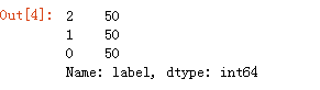
df.label.value_counts()value_counts #计算相同数据出现的次数
In[4]
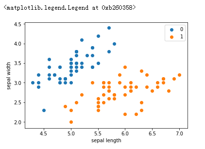
plt.scatter(df[:50]['sepal length'], df[:50]['sepal width'], label='0') #绘制散点图
plt.scatter(df[50:100]['sepal length'], df[50:100]['sepal width'], label='1')
plt.xlabel('sepal length') #给图加上图例
plt.ylabel('sepal width')
plt.legend()
In[5]
data = np.array(df.iloc[:100, [0, 1, -1]])) #按行索引,取出第0,1,-1列
In[6]
X, y = data[:,:-1], data[:,-1] #X为sepal length,sepal width y为标签
In[7]
y = np.array([1 if i == 1 else -1 for i in y]) #将两个类别设重新设置为+1 —1
In[8]
# 数据线性可分,二分类数据
# 此处为一元一次线性方程
class Model:
def __init__(self):
self.w = np.ones(len(data[0])-1, dtype=np.float32)
self.b = 0
self.l_rate = 0.1
# self.data = data
def sign(self, x, w, b):
y = np.dot(x, w) + b
return y
# 随机梯度下降法
def fit(self, X_train, y_train):
is_wrong = False #假设没有误分点
while not is_wrong:
wrong_count = 0
for d in range(len(X_train)):
X = X_train[d]
y = y_train[d]
if y * self.sign(X, self.w, self.b) <= 0: #分类错误
self.w = self.w + self.l_rate*np.dot(y, X) #重新梯度计算w
self.b = self.b + self.l_rate*y #重新梯度计算b
wrong_count += 1
if wrong_count == 0: #通过梯度计算分类分类正确
is_wrong = True
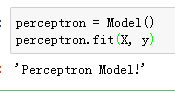
return 'Perceptron Model!'
def score(self):
pass
In[9]
perceptron = Model()
perceptron.fit(X, y) #感知机模型
In[10]
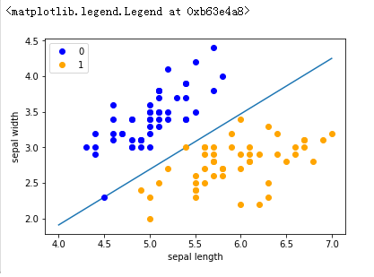
x_points = np.linspace(4, 7,10) #x轴的划分
y_ = -(perceptron.w[0]*x_points + perceptron.b)/perceptron.w[1]
plt.plot(x_points, y_) #绘制模型图像(数据、颜色、图例等信息)
plt.plot(data[:50, 0], data[:50, 1], 'bo', color='blue', label='0')
plt.plot(data[50:100, 0], data[50:100, 1], 'bo', color='orange', label='1')
plt.xlabel('sepal length')
plt.ylabel('sepal width')
plt.legend()
In[11]
from sklearn.linear_model import Perceptron
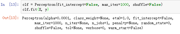
In[12]
clf = Perceptron(fit_intercept=False, max_iter=1000, shuffle=False)
clf.fit(X, y)
In[13]
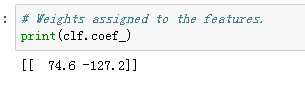
# Weights assigned to the features.
print(clf.coef_)
In[14]
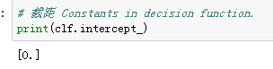
# 截距 Constants in decision function.
print(clf.intercept_)
In[15]
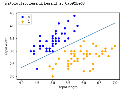
x_ponits = np.arange(4, 8) #确定x轴和y轴的值
y_ = -(clf.coef_[0][0]*x_ponits + clf.intercept_)/clf.coef_[0][1]
plt.plot(x_ponits, y_) #确定拟合的图像的具体信息(数据点,线,大小,粗细颜色等内容)
plt.plot(data[:50, 0], data[:50, 1], 'bo', color='blue', label='0')
plt.plot(data[50:100, 0], data[50:100, 1], 'bo', color='orange', label='1')
plt.xlabel('sepal length')
plt.ylabel('sepal width')
plt.legend()
实验截图:
In[3]
In[4]
In[9]
In[10]
In[12]
In[13]
In[14]
In[15]
五.实验小结
对感知机有了更进一步的学习,通过查阅资料对具体的每行代码有了进一步了解,通过此次实验,对课堂上老师讲的内容进行了巩固。

 浙公网安备 33010602011771号