

akka stream第二课-图
Introduction
In Akka Streams computation graphs are not expressed using a fluent DSL like linear computations are, instead they are written in a more graph-resembling DSL which aims to make translating graph drawings (e.g. from notes taken from design discussions, or illustrations in protocol specifications) to and from code simpler. In this section we’ll dive into the multiple ways of constructing and re-using graphs, as well as explain common pitfalls and how to avoid them.
在Akka流中,计算图不是用流畅的DSL来表示的,线性计算是用更类似DSL的图形编写的,其目的是使图形图形(例如从设计讨论中获得的注释,或协议规范中的插图)与代码之间的转换更简单。在本节中,我们将深入研究构造和重用图的多种方法,并解释常见的陷阱以及如何避免它们。
Graphs are needed whenever you want to perform any kind of fan-in (“multiple inputs”) or fan-out (“multiple outputs”) operations. Considering linear Flows to be like roads, we can picture graph operations as junctions: multiple flows being connected at a single point. Some operators which are common enough and fit the linear style of Flows, such as concat (which concatenates two streams, such that the second one is consumed after the first one has completed), may have shorthand methods defined on Flow or Source themselves, however you should keep in mind that those are also implemented as graph junctions.
无论何时需要执行任何类型的扇入(“多输入”)或扇出(“多输出”)操作,都需要图形。考虑到线性流类似于道路,我们可以将图形操作描绘为交叉点:多个流在一个点上连接。一些足够常见并适合流的线性样式的运算符,例如concat(它连接两个流,以便在第一个流完成后使用第二个流),可能在流或源本身上定义了速记方法,但是您应该记住,这些也是作为图连接实现的。
Dependency
To use Akka Streams, add the module to your project:
要使用Akka Streams,请将模块添加到您的项目中:
val AkkaVersion = "2.6.8"
libraryDependencies += "com.typesafe.akka" %% "akka-stream" % AkkaVersion
Constructing Graphs
构造图Graphs
Graphs are built from simple Flows which serve as the linear connections within the graphs as well as junctions which serve as fan-in and fan-out points for Flows. Thanks to the junctions having meaningful types based on their behavior and making them explicit elements these elements should be rather straightforward to use.
图(Graphs)是由简单的流(Flow)构成的,这些流是图中的线性连接,连接是流的扇入和扇出点。由于连接具有基于其行为的有意义类型,并使其成为显式元素,这些元素的使用应该相当简单。
Akka Streams currently provide these junctions (for a detailed list see the operator index):
Akka Streams现在提供这些交叉点,即图形操作
- Fan-out
-
Broadcast[T](广播)– (1 input, N outputs) given an input element emits to each output 给定一个输入元素向每个输出发射Balance[T]– (1 input, N outputs) given an input element emits to one of its output ports给定一个输入元件发射到它的一个输出端口UnzipWith[In,A,B,...]– (1 input, N outputs) takes a function of 1 input that given a value for each input emits N output elements (where N <= 20)接受一个1个输入的函数,该函数为每个输入给定一个值,会发出N个输出元素(其中N<=20)UnZip[A,B]– (1 input, 2 outputs) splits a stream of(A,B)tuples into two streams, one of typeAand one of typeB将(A,B)元组的流拆分为两个流,一个是类型A,另一个是类型B
- Fan-in
Merge[In](结合)– (N inputs , 1 output) picks randomly from inputs pushing them one by one to its output从输入中随机选取,一个接一个地推送到输出MergePreferred[In]– likeMergebut if elements are available onpreferredport, it picks from it, otherwise randomly fromothers与Merge类似,但如果首选端口上有可用的元素,它将从中选择,否则将从其他端口随机选择MergePrioritized[In]– likeMergebut if elements are available on all input ports, it picks from them randomly based on theirpriority与Merge类似,但如果元素在所有输入端口上都可用,它会根据它们的优先级随机从中选择MergeLatest[In]– (N inputs, 1 output) emitsList[In], when i-th input stream emits element, then i-th element in emitted list is updated发出List[In],当第i个输入流发出元素时,则更新已发出列表中的第i个元素MergeSequence[In]– (N inputs, 1 output) emitsList[In], where the input streams must represent a partitioned sequence that must be merged back together in order发出List[In],其中输入流必须表示一个分区序列,该序列必须按顺序合并在一起ZipWith[A,B,...,Out]– (N inputs, 1 output) which takes a function of N inputs that given a value for each input emits 1 output element它接受N个输入的函数,每个输入给定一个值,发出1个输出元素Zip[A,B]– (2 inputs, 1 output) is aZipWithspecialised to zipping input streams ofAandBinto a(A,B)tuple stream是一个专门用于将A和B的输入流压缩成(A,B)元组流的ZipConcat[A]– (2 inputs, 1 output) concatenates two streams (first consume one, then the second one)串联两个流(首先消耗一个,然后消耗第二个)
One of the goals of the GraphDSL DSL is to look similar to how one would draw a graph on a whiteboard, so that it is simple to translate a design from whiteboard to code and be able to relate those two. Let’s illustrate this by translating the below hand drawn graph into Akka Streams:
GraphDSL DSL的目标之一是看起来类似于在白板上绘制图形的方式,这样就可以很容易地将设计从白板转换为代码,并能够将这两者联系起来。让我们通过将下面的手绘图转换成Akka Streams来说明这一点:
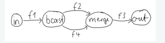
Such graph is simple to translate to the Graph DSL since each linear element corresponds to a Flow, and each circle corresponds to either a Junction or a Source or Sink if it is beginning or ending a Flow. Junctions must always be created with defined type parameters, as otherwise the Nothing type will be inferred.
这样的图很容易转换成DSL图,因为每个线性元素对应于一个流Flow,而每个圆Graphs对应于一个连接或一个源Source或汇Sink(如果它是流的开始或结束)。连接必须始终使用定义的类型参数创建,否则将推断Nothing类型。
val g = RunnableGraph.fromGraph(GraphDSL.create() { implicit builder: GraphDSL.Builder[NotUsed] =>
  import GraphDSL.Implicits._
  val in = Source(1 to 10)
  val out = Sink.ignore

  val bcast = builder.add(Broadcast[Int](2))
  val merge = builder.add(Merge[Int](2))

  val f1, f2, f3, f4 = Flow[Int].map(_ + 10)

  in ~> f1 ~> bcast ~> f2 ~> merge ~> f3 ~> out
  bcast ~> f4 ~> merge
  ClosedShape
})
以上例为模板,重建新的图,同时

val g=RunnableGraph.fromGraph(GraphDSL.create(){implicit buidler=>
    import GraphDSL.Implicits._
    val in=Source(1 to 10)
    val out=Sink.foreach(println)
    val bcast=buidler.add(Broadcast[Int](3))
    val mcast=buidler.add(Merge[Int](3))
    val  f1,f2,f3=Flow[Int].map(_+10)
    val f4=Flow[Int].map(_+0)
    val f5=Flow[Int].map(_+1)
    in ~> f1 ~> bcast ~> f2 ~> mcast ~> f3 ~> out
    bcast ~> f4 ~>mcast
    bcast ~> f5 ~>mcast
    ClosedShape
  })

  g.run()
//31
//21
//22
//32
//22
//23
//33
//23
//24
//34
//24
//25
//35
//25
//26
//36
//26
//27
//37
//27
//28
//38
//28
//29
//39
//29
//30
//40
//30
//31
注意:连接引用相等定义图形节点相等(即,GraphDSL中使用的相同合并实例引用结果图中的相同位置)。
Notice the import GraphDSL.Implicits._ which brings into scope the ~> operator (read as “edge”, “via” or “to”) and its inverted counterpart <~ (for noting down flows in the opposite direction where appropriate).
注意导入GraphDSL.隐式.u将~>运算符(读作“edge”、“via”或“to”)及其倒置的运算符<~(用于在适当的情况下记下流向相反的方向)。
By looking at the snippets above, it should be apparent that the GraphDSL.Builder object is mutable. It is used (implicitly) by the ~> operator, also making it a mutable operation as well. The reason for this design choice is to enable simpler creation of complex graphs, which may even contain cycles. Once the GraphDSL has been constructed though, the GraphDSL instance is immutable, thread-safe, and freely shareable. The same is true of all operators—sources, sinks, and flows—once they are constructed. This means that you can safely re-use one given Flow or junction in multiple places in a processing graph.
通过查看上面的片段,很明显图形生成器对象是可变的。它由~>运算符(隐式地)使用,也使其成为可变操作。这种设计选择的原因是为了能够更简单地创建复杂的图,甚至可能包含循环。但是,一旦GraphDSL被构造出来,
GraphDSL实例是不可变的、线程安全的和可自由共享的。所有操作符的源、汇和流一旦构造好,也是如此。这意味着您可以在处理图的多个位置安全地重用一个给定的流或连接。
We have seen examples of such re-use already above: the merge and broadcast junctions were imported into the graph using builder.add(...), an operation that will make a copy of the blueprint that is passed to it and return the inlets and outlets of the resulting copy so that they can be wired up. Another alternative is to pass existing graphs—of any shape—into the factory method that produces a new graph. The difference between these approaches is that importing using builder.add(...) ignores the materialized value of the imported graph while importing via the factory method allows its inclusion; for more details see Stream Materialization.
我们已经在上面看到了这样的重复使用的例子:合并和广播连接是用builder.add(…),一种操作,它将生成传递给它的蓝图的副本,并返回结果副本的入口和出口,以便将它们连接起来。
另一种方法是将任何形状的现有图形传递到生成新图形的工厂方法中。这些方法之间的区别在于导入时使用生成器.add(…)忽略导入图形的物化值,而通过工厂方法导入时允许包含它;有关更多详细信息,请参阅流物化。
In the example below we prepare a graph that consists of two parallel streams, in which we re-use the same instance of Flow, yet it will properly be materialized as two connections between the corresponding Sources and Sinks:
在下面的示例中,我们准备了一个由两个并行流组成的图,在这个图中,我们重用了相同的Flow实例,但它将被适当地具体化为相应的源和汇之间的两个连接:
val topHeadSink = Sink.head[Int]
val bottomHeadSink = Sink.head[Int]
val sharedDoubler = Flow[Int].map(_ * 2)

RunnableGraph.fromGraph(GraphDSL.create(topHeadSink, bottomHeadSink)((_, _)) { implicit builder =>
  (topHS, bottomHS) =>
  import GraphDSL.Implicits._
  val broadcast = builder.add(Broadcast[Int](2))
  Source.single(1) ~> broadcast.in

  broadcast ~> sharedDoubler ~> topHS.in
  broadcast ~> sharedDoubler ~> bottomHS.in
  ClosedShape
})
案例2:
  val topHeadSink = Sink.head[Int]
  val bottomHeadSink = Sink.head[Int]
  val sharedDoubler = Flow[Int].map(_ * 2)

  val srun:(Future[Int],Future[Int])=RunnableGraph.fromGraph(GraphDSL.create(topHeadSink, bottomHeadSink)((_, _)) { implicit builder =>
    (topHS, bottomHS) =>
      import GraphDSL.Implicits._
      val broadcast = builder.add(Broadcast[Int](2))
      Source.single(1) ~> broadcast.in
      broadcast ~> sharedDoubler ~> topHS.in
      broadcast ~> sharedDoubler ~> bottomHS.in
      ClosedShape
  }).run()

println(Await.result(srun._1,3 seconds))
In some cases we may have a list of graph elements, for example if they are dynamically created. If these graphs have similar signatures, we can construct a graph collecting all their materialized values as a collection:
在某些情况下,我们可能会有一个图元素的列表,例如,如果它们是动态创建的。如果这些图具有相似的签名,我们可以构造一个图,将它们的所有物化值收集为一个集合:
import scala.collection._
  val sinks = immutable
  .Seq("a", "b", "c")
  .map(prefix => Flow[String].filter(str => str.startsWith(prefix)).toMat(Sink.head[String])(Keep.right))

  val g: RunnableGraph[Seq[Future[String]]] = RunnableGraph.fromGraph(GraphDSL.create(sinks) {
    implicit b => sinkList =>
      import GraphDSL.Implicits._
      val broadcast = b.add(Broadcast[String](sinkList.size))

      Source(List("ax", "bx", "cx")) ~> broadcast
      sinkList.foreach(sink => broadcast ~> sink)

      ClosedShape
  })

  val matList: Seq[Future[String]] = g.run()
  val format=matList.map(a=>Await.result(a,3 seconds))
  println(format)//List(ax, bx, cx)
val sw=Await.result(Future.sequence(matList),3 seconds)//sequence是将Seq[Future]=>Future[Seq]的方法
println(sw)//List(ax, bx, cx)
Constructing and combining Partial Graphs
局部图的构造与组合
Sometimes it is not possible (or needed) to construct the entire computation graph in one place, but instead construct all of its different phases in different places and in the end connect them all into a complete graph and run it.
有时不可能(或不需要)在一个地方构造整个计算图,而是在不同的地方构造它的所有不同阶段,最后将它们连接成一个完整的图并运行它。
This can be achieved by returning a different Shape than ClosedShape, for example FlowShape(in, out), from the function given to GraphDSL.create. See Predefined shapes for a list of such predefined shapes. Making a Graph a RunnableGraph requires all ports to be connected, and if they are not it will throw an exception at construction time, which helps to avoid simple wiring errors while working with graphs. A partial graph however allows you to return the set of yet to be connected ports from the code block that performs the internal wiring.
这可以通过返回与ClosedShape不同的形状来实现,例如FlowShape(in,out),从给定的函数返回GraphDSL.create.创建. 有关此类预定义形状的列表,请参见预定义形状。使一个图形成为一个RunnableGraph需要连接所有端口,如果没有,它将在构造时抛出一个异常,这有助于避免在处理图形时出现简单的布线错误。但是,局部图允许您从执行内部连接的代码块返回尚未连接的端口集。
Let’s imagine we want to provide users with a specialized element that given 3 inputs will pick the greatest int value of each zipped triple. We’ll want to expose 3 input ports (unconnected sources) and one output port (unconnected sink).
假设我们想为用户提供一个特殊的元素,给定3个输入将选择每个压缩三元组的最大int值。我们需要公开3个输入端口(未连接的源)和一个输出端口(未连接的sink)。
val pickMaxOfThree = GraphDSL.create() { implicit b =>
  import GraphDSL.Implicits._

  val zip1 = b.add(ZipWith[Int, Int, Int](math.max _))
  val zip2 = b.add(ZipWith[Int, Int, Int](math.max _))
  zip1.out ~> zip2.in0

  UniformFanInShape(zip2.out, zip1.in0, zip1.in1, zip2.in1)
}

val resultSink = Sink.head[Int]

val g = RunnableGraph.fromGraph(GraphDSL.create(resultSink) { implicit b => sink =>
  import GraphDSL.Implicits._

  // importing the partial graph will return its shape (inlets & outlets)
  val pm3 = b.add(pickMaxOfThree)

  Source.single(1) ~> pm3.in(0)
  Source.single(2) ~> pm3.in(1)
  Source.single(3) ~> pm3.in(2)
  pm3.out ~> sink.in
  ClosedShape
})

val max: Future[Int] = g.run()
Await.result(max, 300.millis) should equal(3)
ZipWiths, in reality ZipWith already provides numerous overloads including a 3 (and many more) parameter versions. So this could be implemented using one ZipWith using the 3 parameter version, like this: ZipWith((a, b, c) => out). (The ZipWith with N input has N+1 type parameter; the last type param is the output type.)注意:虽然上面的例子展示了如何组合两个2输入ZipWith,但实际上ZipWith已经提供了许多重载,包括一个3(以及更多)参数版本。所以这可以用一个ZipWith实现,使用3个参数版本,比如:ZipWith((a,b,c)=>out)。(具有N个输入的ZipWith具有N+1个类型参数;最后一个类型参数是输出类型。)
As you can see, first we construct the partial graph that contains all the zipping and comparing of stream elements. This partial graph will have three inputs and one output, wherefore we use the UniformFanInShape. Then we import it (all of its nodes and connections) explicitly into the closed graph built in the second step in which all the undefined elements are rewired to real sources and sinks. The graph can then be run and yields the expected result.
如您所见,首先我们构建了包含流元素的所有压缩和比较的部分图。这个部分图将有三个输入和一个输出,因此我们使用uniformfanishape。然后我们将它(它的所有节点和连接)显式地导入到第二步构建的封闭图中,在这个图中,所有未定义的元素都被重新连接到真实的源和汇。然后可以运行该图并生成预期结果。
GraphDSL is not able to provide compile time type-safety about whether or not all elements have been properly connected—this validation is performed as a runtime check during the graph’s instantiation.警告:请注意,GraphDSL不能提供关于是否所有元素都已正确连接的编译时类型安全性此验证在图的实例化期间作为运行时检查执行。
A partial graph also verifies that all ports are either connected or part of the returned Shape.
部分图还验证所有端口是否已连接或是返回形状的一部分。
Constructing Sources, Sinks and Flows from Partial Graphs
从局部图构造源、汇和流
Instead of treating a partial graph as a collection of flows and junctions which may not yet all be connected it is sometimes useful to expose such a complex graph as a simpler structure, such as a Source, Sink or Flow.
与其将部分图视为尚未全部连接的流和连接的集合,不如将这种复杂的图公开为更简单的结构,例如源、汇或流。
In fact, these concepts can be expressed as special cases of a partially connected graph:
实际上,这些概念可以表示为部分连通图的特例:
Sourceis a partial graph with exactly one output, that is it returns aSourceShape.
Source是一个只有一个输出的部分图,即它返回一个SourceShape。
Sinkis a partial graph with exactly one input, that is it returns aSinkShape.
Sink是一个只有一个输入的部分图,即返回SinkShape。
Flowis a partial graph with exactly one input and exactly one output, that is it returns aFlowShape.
Flow是一个只有一个输入和一个输出的部分图,即它返回一个FlowShape。
Being able to hide complex graphs inside of simple elements such as Sink / Source / Flow enables you to create one complex element and from there on treat it as simple compound operator for linear computations.
能够将复杂的图形隐藏在简单元素(如Sink/Source/Flow)中,可以创建一个复杂元素,然后将其视为线性计算的简单复合运算符。
In order to create a Source from a graph the method Source.fromGraph is used, to use it we must have a Graph[SourceShape, T]. This is constructed using GraphDSL.create and returning a SourceShape from the function passed in. The single outlet must be provided to the SourceShape.of method and will become “the sink that must be attached before this Source can run”.
为了从图中创建源,使用Source.fromGraph方法,我们必须有一个图形[SourceShape,T]。这是用GraphDSL.create.创建并从传入的函数返回SourceShape。必须为SourceShape.of方法,并将成为“运行此源之前必须附加的接收器”。
Refer to the example below, in which we create a Source that zips together two numbers, to see this graph construction in action:
请参阅下面的示例,在该示例中,我们创建了一个将两个数字压缩在一起的源,以查看此图形构造的实际操作:
val pairs = Source.fromGraph(GraphDSL.create() { implicit b =>
  import GraphDSL.Implicits._

  // prepare graph elements
  val zip = b.add(Zip[Int, Int]())
  def ints = Source.fromIterator(() => Iterator.from(1))

  // connect the graph
  ints.filter(_ % 2 != 0) ~> zip.in0
  ints.filter(_ % 2 == 0) ~> zip.in1

  // expose port
  SourceShape(zip.out)
})

val firstPair: Future[(Int, Int)] = pairs.runWith(Sink.head)
Similarly the same can be done for a Sink[T], using SinkShape.of in which case the provided value must be an Inlet[T]. For defining a Flow[T] we need to expose both an inlet and an outlet:
同样地,对于Sink[T],也可以使用SinkShape.of在这种情况下,提供的值必须是Inlet[T]。为了定义Flow[T],我们需要同时暴露入口和出口:
val pairUpWithToString =
  Flow.fromGraph(GraphDSL.create() { implicit b =>
    import GraphDSL.Implicits._

    // prepare graph elements
    val broadcast = b.add(Broadcast[Int](2))
    val zip = b.add(Zip[Int, String]())

    // connect the graph
    broadcast.out(0).map(identity) ~> zip.in0
    broadcast.out(1).map(_.toString) ~> zip.in1

    // expose ports
    FlowShape(broadcast.in, zip.out)
  })

pairUpWithToString.runWith(Source(List(1)), Sink.head)
Combining Sources and Sinks with simplified API
使用简化的API组合源和汇
There is a simplified API you can use to combine sources and sinks with junctions like: Broadcast[T], Balance[T], Merge[In] and Concat[A] without the need for using the Graph DSL. The combine method takes care of constructing the necessary graph underneath. In following example we combine two sources into one (fan-in):
有一个简化的API可以用来将源和汇与连接结合起来,比如:Broadcast[T]、Balance[T]、Merge[In]和Concat[a],而不需要使用Graph DSL。组合方法负责在下面构造必要的图。在下面的示例中,我们将两个源合并为一个(扇入):
val sourceOne = Source(List(1))
val sourceTwo = Source(List(2))
val merged = Source.combine(sourceOne, sourceTwo)(Merge(_))

val mergedResult: Future[Int] = merged.runWith(Sink.fold(0)(_ + _))
The same can be done for a Sink[T] but in this case it will be fan-out:
Sink[T]也可以这样做,但在这种情况下,它将扇出:
val sendRmotely = Sink.actorRef(actorRef, "Done", _ => "Failed")
val localProcessing = Sink.foreach[Int](_ => /* do something useful */ ())

val sink = Sink.combine(sendRmotely, localProcessing)(Broadcast[Int](_))

Source(List(0, 1, 2)).runWith(sink)
Building reusable Graph components
构建可重用的图形组件
It is possible to build reusable, encapsulated components of arbitrary input and output ports using the graph DSL.
使用图形DSL可以构建任意输入和输出端口的可重用封装组件。
As an example, we will build a graph junction that represents a pool of workers, where a worker is expressed as a Flow[I,O,_], i.e. a simple transformation of jobs of type I to results of type O (as you have seen already, this flow can actually contain a complex graph inside). Our reusable worker pool junction will not preserve the order of the incoming jobs (they are assumed to have a proper ID field) and it will use a Balance junction to schedule jobs to available workers. On top of this, our junction will feature a “fastlane”, a dedicated port where jobs of higher priority can be sent.
例如,我们将构建一个表示worker池的graph junction,其中worker被表示为Flow[I,O,_],即将类型I的作业简单转换为类型O的结果(正如您已经看到的,这个流实际上可以包含一个复杂的图)。我们的可重用worker池连接将不保留传入作业的顺序(假定它们具有正确的ID字段),它将使用Balance连接将作业调度给可用的工人。除此之外,我们的交叉口将有一个“快车道”,一个可以发送高优先级工作的专用端口。
Altogether, our junction will have two input ports of type I (for the normal and priority jobs) and an output port of type O. To represent this interface, we need to define a custom Shape. The following lines show how to do that.
总之,我们的连接将有两个I型输入端口(用于普通和优先级作业)和一个O型输出端口。要表示此接口,我们需要定义一个自定义形状。下面的几行代码展示了如何做到这一点。
// A shape represents the input and output ports of a reusable
// processing module
case class PriorityWorkerPoolShape[In, Out](jobsIn: Inlet[In], priorityJobsIn: Inlet[In], resultsOut: Outlet[Out])
    extends Shape {

  // It is important to provide the list of all input and output
  // ports with a stable order. Duplicates are not allowed.
  override val inlets: immutable.Seq[Inlet[_]] =
    jobsIn :: priorityJobsIn :: Nil
  override val outlets: immutable.Seq[Outlet[_]] =
    resultsOut :: Nil

  // A Shape must be able to create a copy of itself. Basically
  // it means a new instance with copies of the ports
  override def deepCopy() =
    PriorityWorkerPoolShape(jobsIn.carbonCopy(), priorityJobsIn.carbonCopy(), resultsOut.carbonCopy())

}
Predefined shapes
预定义形状
In general a custom Shape needs to be able to provide all its input and output ports, be able to copy itself, and also be able to create a new instance from given ports. There are some predefined shapes provided to avoid unnecessary boilerplate:
一般来说,自定义形状需要能够提供其所有输入和输出端口,能够复制自身,并且能够从给定端口创建新实例。提供了一些预定义的形状,以避免不必要的样板:
SourceShape,SinkShape,FlowShapefor simpler shapes,SourceShape、SinkShape、FlowShape用于更简单的形状,
UniformFanInShapeandUniformFanOutShapefor junctions with multiple input (or output) ports of the same type,
UniformFanInShape和UniformFanOutShape用于具有相同类型的多个输入(或输出)端口的连接,FanInShape1,FanInShape2, …,FanOutShape1,FanOutShape2, … for junctions with multiple input (or output) ports of different types.FanInShape1,FanInShape2,…,fanutshape1,fanutshape2,…,用于具有不同类型的多个输入(或输出)端口的连接。
Since our shape has two input ports and one output port, we can use the FanInShape DSL to define our custom shape:
因为我们的形状有两个输入端口和一个输出端口,所以我们可以使用FanInShape DSL来定义我们的自定义形状:
import FanInShape.{ Init, Name }

class PriorityWorkerPoolShape2[In, Out](_init: Init[Out] = Name("PriorityWorkerPool"))
    extends FanInShape[Out](_init) {
  protected override def construct(i: Init[Out]) = new PriorityWorkerPoolShape2(i)

  val jobsIn = newInlet[In]("jobsIn")
  val priorityJobsIn = newInlet[In]("priorityJobsIn")
  // Outlet[Out] with name "out" is automatically created
}
Now that we have a Shape we can wire up a Graph that represents our worker pool. First, we will merge incoming normal and priority jobs using MergePreferred, then we will send the jobs to a Balance junction which will fan-out to a configurable number of workers (flows), finally we merge all these results together and send them out through our only output port. This is expressed by the following code:
现在我们有了一个形状,我们可以连接一个表示我们的工人池的图形。首先,我们将使用MergePreferred合并传入的普通作业和优先级作业,然后将作业发送到一个平衡连接点,该连接点将扇出可配置数量的工人(流),最后我们将所有这些结果合并在一起,并通过我们唯一的输出端口发送出去。这由以下代码表示:
object PriorityWorkerPool {
  def apply[In, Out](
      worker: Flow[In, Out, Any],
      workerCount: Int): Graph[PriorityWorkerPoolShape[In, Out], NotUsed] = {

    GraphDSL.create() { implicit b =>
      import GraphDSL.Implicits._

      val priorityMerge = b.add(MergePreferred[In](1))
      val balance = b.add(Balance[In](workerCount))
      val resultsMerge = b.add(Merge[Out](workerCount))

      // After merging priority and ordinary jobs, we feed them to the balancer
      priorityMerge ~> balance

      // Wire up each of the outputs of the balancer to a worker flow
      // then merge them back
      for (i <- 0 until workerCount)
        balance.out(i) ~> worker ~> resultsMerge.in(i)

      // We now expose the input ports of the priorityMerge and the output
      // of the resultsMerge as our PriorityWorkerPool ports
      // -- all neatly wrapped in our domain specific Shape
      PriorityWorkerPoolShape(
        jobsIn = priorityMerge.in(0),
        priorityJobsIn = priorityMerge.preferred,
        resultsOut = resultsMerge.out)
    }

  }

}
All we need to do now is to use our custom junction in a graph. The following code simulates some simple workers and jobs using plain strings and prints out the results. Actually we used two instances of our worker pool junction using add() twice.
我们现在需要做的就是在图中使用我们的自定义连接。下面的代码使用纯字符串模拟一些简单的工人和作业,并输出结果。实际上,我们两次使用add()来使用worker池连接的两个实例。
val worker1 = Flow[String].map("step 1 " + _)
val worker2 = Flow[String].map("step 2 " + _)

RunnableGraph
  .fromGraph(GraphDSL.create() { implicit b =>
    import GraphDSL.Implicits._

    val priorityPool1 = b.add(PriorityWorkerPool(worker1, 4))
    val priorityPool2 = b.add(PriorityWorkerPool(worker2, 2))

    Source(1 to 100).map("job: " + _) ~> priorityPool1.jobsIn
    Source(1 to 100).map("priority job: " + _) ~> priorityPool1.priorityJobsIn

    priorityPool1.resultsOut ~> priorityPool2.jobsIn
    Source(1 to 100).map("one-step, priority " + _) ~> priorityPool2.priorityJobsIn

    priorityPool2.resultsOut ~> Sink.foreach(println)
    ClosedShape
  })
  .run()
Bidirectional Flows
双向流动
A graph topology that is often useful is that of two flows going in opposite directions. Take for example a codec operator that serializes outgoing messages and deserializes incoming octet streams. Another such operator could add a framing protocol that attaches a length header to outgoing data and parses incoming frames back into the original octet stream chunks. These two operators are meant to be composed, applying one atop the other as part of a protocol stack. For this purpose exists the special type BidiFlow which is a graph that has exactly two open inlets and two open outlets. The corresponding shape is called BidiShape and is defined like this:
通常有用的图拓扑是两个流向相反方向的流。以一个编解码器操作符为例,它序列化传出消息并反序列化传入的八位字节流。另一个这样的运算符可以添加一个帧协议,该协议将一个长度头附加到传出数据,并将传入的帧解析回原始的八位字节流块。这两个操作符应该组合在一起,作为协议栈的一部分应用于另一个之上。为此,存在一个特殊类型的BidiFlow,它是一个正好有两个开放入口和两个开放出口的图形。相应的形状称为BidiShape,其定义如下:
/**
 * A bidirectional flow of elements that consequently has two inputs and two
 * outputs, arranged like this:
 *
 * {{{
 *        +------+
 *  In1 ~>|      |~> Out1
 *        | bidi |
 * Out2 <~|      |<~ In2
 *        +------+
 * }}}
 */
final case class BidiShape[-In1, +Out1, -In2, +Out2](
    in1: Inlet[In1 @uncheckedVariance],
    out1: Outlet[Out1 @uncheckedVariance],
    in2: Inlet[In2 @uncheckedVariance],
    out2: Outlet[Out2 @uncheckedVariance])
    extends Shape {
  override val inlets: immutable.Seq[Inlet[_]] = in1 :: in2 :: Nil
  override val outlets: immutable.Seq[Outlet[_]] = out1 :: out2 :: Nil

  /**
   * Java API for creating from a pair of unidirectional flows.
   */
  def this(top: FlowShape[In1, Out1], bottom: FlowShape[In2, Out2]) = this(top.in, top.out, bottom.in, bottom.out)

  override def deepCopy(): BidiShape[In1, Out1, In2, Out2] =
    BidiShape(in1.carbonCopy(), out1.carbonCopy(), in2.carbonCopy(), out2.carbonCopy())

}
A bidirectional flow is defined just like a unidirectional Flow as demonstrated for the codec mentioned above:
双向流的定义与单向流的定义相同,如上述编解码器所示:
trait Message
case class Ping(id: Int) extends Message
case class Pong(id: Int) extends Message

def toBytes(msg: Message): ByteString = {
  implicit val order = ByteOrder.LITTLE_ENDIAN
  msg match {
    case Ping(id) => ByteString.newBuilder.putByte(1).putInt(id).result()
    case Pong(id) => ByteString.newBuilder.putByte(2).putInt(id).result()
  }
}

def fromBytes(bytes: ByteString): Message = {
  implicit val order = ByteOrder.LITTLE_ENDIAN
  val it = bytes.iterator
  it.getByte match {
    case 1     => Ping(it.getInt)
    case 2     => Pong(it.getInt)
    case other => throw new RuntimeException(s"parse error: expected 1|2 got $other")
  }
}

val codecVerbose = BidiFlow.fromGraph(GraphDSL.create() { b =>
  // construct and add the top flow, going outbound
  val outbound = b.add(Flow[Message].map(toBytes))
  // construct and add the bottom flow, going inbound
  val inbound = b.add(Flow[ByteString].map(fromBytes))
  // fuse them together into a BidiShape
  BidiShape.fromFlows(outbound, inbound)
})

// this is the same as the above
val codec = BidiFlow.fromFunctions(toBytes _, fromBytes _)
The first version resembles the partial graph constructor, while for the simple case of a functional 1:1 transformation there is a concise convenience method as shown on the last line. The implementation of the two functions is not difficult either:
第一个版本类似于部分图构造函数,而对于函数1:1转换的简单情况,有一个简明的方便方法,如最后一行所示。这两项职能的实施也并不困难:
def toBytes(msg: Message): ByteString = {
  implicit val order = ByteOrder.LITTLE_ENDIAN
  msg match {
    case Ping(id) => ByteString.newBuilder.putByte(1).putInt(id).result()
    case Pong(id) => ByteString.newBuilder.putByte(2).putInt(id).result()
  }
}

def fromBytes(bytes: ByteString): Message = {
  implicit val order = ByteOrder.LITTLE_ENDIAN
  val it = bytes.iterator
  it.getByte match {
    case 1     => Ping(it.getInt)
    case 2     => Pong(it.getInt)
    case other => throw new RuntimeException(s"parse error: expected 1|2 got $other")
  }
}
In this way you can integrate any other serialization library that turns an object into a sequence of bytes.
通过这种方式,您可以集成任何其他将对象转换为字节序列的序列化库。
The other operator that we talked about is a little more involved since reversing a framing protocol means that any received chunk of bytes may correspond to zero or more messages. This is best implemented using GraphStage (see also Custom processing with GraphStage).
我们讨论的另一个操作符则涉及的更多,因为反转帧协议意味着任何接收到的字节块都可能对应于零个或多个消息。这最好使用GraphStage实现(另请参见GraphStage的自定义处理)。
val framing = BidiFlow.fromGraph(GraphDSL.create() { b =>
  implicit val order = ByteOrder.LITTLE_ENDIAN

  def addLengthHeader(bytes: ByteString) = {
    val len = bytes.length
    ByteString.newBuilder.putInt(len).append(bytes).result()
  }

  class FrameParser extends GraphStage[FlowShape[ByteString, ByteString]] {

    val in = Inlet[ByteString]("FrameParser.in")
    val out = Outlet[ByteString]("FrameParser.out")
    override val shape = FlowShape.of(in, out)

    override def createLogic(inheritedAttributes: Attributes): GraphStageLogic = new GraphStageLogic(shape) {

      // this holds the received but not yet parsed bytes
      var stash = ByteString.empty
      // this holds the current message length or -1 if at a boundary
      var needed = -1

      setHandler(out, new OutHandler {
        override def onPull(): Unit = {
          if (isClosed(in)) run()
          else pull(in)
        }
      })
      setHandler(in, new InHandler {
        override def onPush(): Unit = {
          val bytes = grab(in)
          stash = stash ++ bytes
          run()
        }

        override def onUpstreamFinish(): Unit = {
          // either we are done
          if (stash.isEmpty) completeStage()
          // or we still have bytes to emit
          // wait with completion and let run() complete when the
          // rest of the stash has been sent downstream
          else if (isAvailable(out)) run()
        }
      })

      private def run(): Unit = {
        if (needed == -1) {
          // are we at a boundary? then figure out next length
          if (stash.length < 4) {
            if (isClosed(in)) completeStage()
            else pull(in)
          } else {
            needed = stash.iterator.getInt
            stash = stash.drop(4)
            run() // cycle back to possibly already emit the next chunk
          }
        } else if (stash.length < needed) {
          // we are in the middle of a message, need more bytes,
          // or have to stop if input closed
          if (isClosed(in)) completeStage()
          else pull(in)
        } else {
          // we have enough to emit at least one message, so do it
          val emit = stash.take(needed)
          stash = stash.drop(needed)
          needed = -1
          push(out, emit)
        }
      }
    }
  }

  val outbound = b.add(Flow[ByteString].map(addLengthHeader))
  val inbound = b.add(Flow[ByteString].via(new FrameParser))
  BidiShape.fromFlows(outbound, inbound)
})
With these implementations we can build a protocol stack and test it:
通过这些实现,我们可以构建一个协议栈并对其进行测试:
/* construct protocol stack
 *         +------------------------------------+
 *         | stack                              |
 *         |                                    |
 *         |  +-------+            +---------+  |
 *    ~>   O~~o       |     ~>     |         o~~O    ~>
 * Message |  | codec | ByteString | framing |  | ByteString
 *    <~   O~~o       |     <~     |         o~~O    <~
 *         |  +-------+            +---------+  |
 *         +------------------------------------+
 */
val stack = codec.atop(framing)

// test it by plugging it into its own inverse and closing the right end
val pingpong = Flow[Message].collect { case Ping(id) => Pong(id) }
val flow = stack.atop(stack.reversed).join(pingpong)
val result = Source((0 to 9).map(Ping)).via(flow).limit(20).runWith(Sink.seq)
Await.result(result, 1.second) should ===((0 to 9).map(Pong))
This example demonstrates how BidiFlow subgraphs can be hooked together and also turned around with the .reversed method. The test simulates both parties of a network communication protocol without actually having to open a network connection—the flows can be connected directly.
这个例子演示了如何将BidiFlow子图挂接在一起,也可以使用.reversed方法进行转换。该测试模拟网络通信协议的双方,而无需实际打开网络连接-流可以直接连接。
Accessing the materialized value inside the Graph
访问图中的物化值
In certain cases it might be necessary to feed back the materialized value of a Graph (partial, closed or backing a Source, Sink, Flow or BidiFlow). This is possible by using builder.materializedValue which gives an Outlet that can be used in the graph as an ordinary source or outlet, and which will eventually emit the materialized value. If the materialized value is needed at more than one place, it is possible to call materializedValue any number of times to acquire the necessary number of outlets.
在某些情况下,可能需要反馈图的物化值(部分、封闭或支持源、汇、流或BidiFlow)。这可以通过使用builder.materializedValue它提供了一个出口,可以在图中用作普通的源或出口,并且最终将发出物化值。如果在多个地方需要物化值,则可以多次调用物化值以获得所需数量的出口。
import GraphDSL.Implicits._
val foldFlow: Flow[Int, Int, Future[Int]] = Flow.fromGraph(GraphDSL.create(Sink.fold[Int, Int](0)(_ + _)) {
  implicit builder => fold =>
    FlowShape(fold.in, builder.materializedValue.mapAsync(4)(identity).outlet)
})
Be careful not to introduce a cycle where the materialized value actually contributes to the materialized value. The following example demonstrates a case where the materialized Future of a fold is fed back to the fold itself.
注意不要引入物化价值实际上对物化价值有贡献的循环。下面的例子演示了一个例子,其中一个褶皱的物化未来被反馈到褶皱本身。
import GraphDSL.Implicits._
// This cannot produce any value:
val cyclicFold: Source[Int, Future[Int]] =
  Source.fromGraph(GraphDSL.create(Sink.fold[Int, Int](0)(_ + _)) { implicit builder => fold =>
    // - Fold cannot complete until its upstream mapAsync completes
    // - mapAsync cannot complete until the materialized Future produced by
    //   fold completes
    // As a result this Source will never emit anything, and its materialited
    // Future will never complete
    builder.materializedValue.mapAsync(4)(identity) ~> fold
    SourceShape(builder.materializedValue.mapAsync(4)(identity).outlet)
  })
Graph cycles, liveness and deadlocks
图的循环、活性和死锁
Cycles in bounded stream topologies need special considerations to avoid potential deadlocks and other liveness issues. This section shows several examples of problems that can arise from the presence of feedback arcs in stream processing graphs.
有界流拓扑中的循环需要特别考虑,以避免潜在的死锁和其他活跃性问题。在这一段的反馈图中可以出现几个弧段的问题。
In the following examples runnable graphs are created but do not run because each have some issue and will deadlock after start. Source variable is not defined as the nature and number of element does not matter for described problems.
在下面的示例中,创建了可运行的图,但不运行,因为每个图都有一些问题,并且在启动后会死锁。问题的来源是不定数的,不为数元的性质所描述。
The first example demonstrates a graph that contains a naïve cycle. The graph takes elements from the source, prints them, then broadcasts those elements to a consumer (we just used Sink.ignore for now) and to a feedback arc that is merged back into the main stream via a Merge junction.
第一个示例演示了一个包含天真循环的图。图形从源中获取元素,打印它们,然后将这些元素广播给消费者(我们刚刚使用Sink.忽略现在)和一个反馈弧,它通过一个汇合路口汇入主流。
注意:图形DSL允许反转连接箭头,这在编写周期时特别方便,因为我们将看到在某些情况下这是非常有用的。
// WARNING! The graph below deadlocks!
RunnableGraph.fromGraph(GraphDSL.create() { implicit b =>
  import GraphDSL.Implicits._

  val merge = b.add(Merge[Int](2))
  val bcast = b.add(Broadcast[Int](2))

  source ~> merge ~> Flow[Int].map { s => println(s); s } ~> bcast ~> Sink.ignore
            merge                    <~                      bcast
  ClosedShape
})
Running this we observe that after a few numbers have been printed, no more elements are logged to the console - all processing stops after some time. After some investigation we observe that:
运行这个程序,我们观察到在打印了一些数字之后,没有更多的元素被记录到控制台—所有的处理都会在一段时间后停止。经过一番调查,我们发现:
- through merging from
sourcewe increase the number of elements flowing in the cycle
通过从源代码合并,我们增加了循环中流动的元素的数量
- by broadcasting back to the cycle we do not decrease the number of elements in the cycle
通过广播回周期,我们不会减少周期中的元素数量
Since Akka Streams (and Reactive Streams in general) guarantee bounded processing (see the “Buffering” section for more details) it means that only a bounded number of elements are buffered over any time span. Since our cycle gains more and more elements, eventually all of its internal buffers become full, backpressuring source forever. To be able to process more elements from source elements would need to leave the cycle somehow.
由于Akka流(和一般的反应流)保证有界处理(请参阅“缓冲”部分了解更多详细信息),这意味着在任何时间跨度内只有有限数量的元素被缓冲。由于我们的周期获得了越来越多的元素,最终它的所有内部缓冲区都会变满,永远背压源。为了能够从源元素处理更多的元素,需要以某种方式离开循环。
If we modify our feedback loop by replacing the Merge junction with a MergePreferred we can avoid the deadlock. MergePreferred is unfair as it always tries to consume from a preferred input port if there are elements available before trying the other lower priority input ports. Since we feed back through the preferred port it is always guaranteed that the elements in the cycles can flow.
如果我们通过用MergePreferred替换Merge连接来修改反馈循环,我们可以避免死锁。MergePreferred是不公平的,因为在尝试其他低优先级输入端口之前,如果有可用的元素,它总是尝试从首选输入端口消耗。由于我们通过首选端口反馈,因此始终保证循环中的元素可以流动。
// WARNING! The graph below stops consuming from "source" after a few steps
RunnableGraph.fromGraph(GraphDSL.create() { implicit b =>
  import GraphDSL.Implicits._

  val merge = b.add(MergePreferred[Int](1))
  val bcast = b.add(Broadcast[Int](2))

  source ~> merge ~> Flow[Int].map { s => println(s); s } ~> bcast ~> Sink.ignore
            merge.preferred              <~                  bcast
  ClosedShape
})
If we run the example we see that the same sequence of numbers are printed over and over again, but the processing does not stop. Hence, we avoided the deadlock, but source is still back-pressured forever, because buffer space is never recovered: the only action we see is the circulation of a couple of initial elements from source.
如果我们运行这个例子,我们会看到相同的数字序列被反复打印,但是处理并没有停止。因此,我们避免了僵局,但源仍然永远背压,因为缓冲空间永远无法恢复:我们看到的唯一动作是源中几个初始元素的循环。
注意:我们在这里看到的是,在某些情况下,我们需要在有界和有活力之间作出选择。如果循环中存在无限缓冲区,我们的第一个示例不会死锁,反之亦然,如果循环中的元素是平衡的(移除的元素越多,注入的元素越多),那么就不会出现死锁。
To make our cycle both live (not deadlocking) and fair we can introduce a dropping element on the feedback arc. In this case we chose the buffer() operation giving it a dropping strategy OverflowStrategy.dropHead.
为了使我们的循环既有效又公平,我们可以在反馈弧上引入一个下降元素。在本例中,我们选择了buffer()操作,为它提供了一个删除策略溢出策略.dropHead.
RunnableGraph.fromGraph(GraphDSL.create() { implicit b =>
  import GraphDSL.Implicits._

  val merge = b.add(Merge[Int](2))
  val bcast = b.add(Broadcast[Int](2))

  source ~> merge ~> Flow[Int].map { s => println(s); s } ~> bcast ~> Sink.ignore
      merge <~ Flow[Int].buffer(10, OverflowStrategy.dropHead) <~ bcast
  ClosedShape
})
If we run this example we see that
如果我们运行这个例子,我们会看到
- The flow of elements does not stop, there are always elements printed
元素的流动不会停止,总会有元素被打印出来
- We see that some of the numbers are printed several times over time (due to the feedback loop) but on average the numbers are increasing in the long term
我们看到一些数字随着时间的推移打印了好几次(由于反馈循环),但从长期来看,这些数字平均都在增加
This example highlights that one solution to avoid deadlocks in the presence of potentially unbalanced cycles (cycles where the number of circulating elements are unbounded) is to drop elements. An alternative would be to define a larger buffer with OverflowStrategy.fail which would fail the stream instead of deadlocking it after all buffer space has been consumed.
这个例子强调了一个避免在存在潜在不平衡循环(循环元素的数量是无限的循环)时出现死锁的解决方案是删除元素。另一种方法是使用溢出策略失败这将使流失败,而不是在所有缓冲区空间用完后死锁它。
As we discovered in the previous examples, the core problem was the unbalanced nature of the feedback loop. We circumvented this issue by adding a dropping element, but now we want to build a cycle that is balanced from the beginning instead. To achieve this we modify our first graph by replacing the Merge junction with a ZipWith. Since ZipWith takes one element from source and from the feedback arc to inject one element into the cycle, we maintain the balance of elements.
正如我们在前面的例子中发现的,核心问题是反馈回路的不平衡性。我们通过添加一个droping元素来避免这个问题,但是现在我们想构建一个从一开始就平衡的循环。为了实现这一点,我们修改我们的第一个图,用ZipWith替换合并连接。由于ZipWith从源和反馈弧中提取一个元素,将一个元素注入循环中,因此我们保持了元素的平衡。
// WARNING! The graph below never processes any elements
RunnableGraph.fromGraph(GraphDSL.create() { implicit b =>
  import GraphDSL.Implicits._

  val zip = b.add(ZipWith[Int, Int, Int]((left, right) => right))
  val bcast = b.add(Broadcast[Int](2))

  source ~> zip.in0
  zip.out.map { s => println(s); s } ~> bcast ~> Sink.ignore
  zip.in1             <~                bcast
  ClosedShape
})
Still, when we try to run the example it turns out that no element is printed at all! After some investigation we realize that:
不过,当我们试着运行这个例子时,却发现根本没有元素被打印出来!经过一番调查,我们发现:
- In order to get the first element from
sourceinto the cycle we need an already existing element in the cycle
为了让第一个元素从源代码进入循环,我们需要一个已经存在于循环中的元素
- In order to get an initial element in the cycle we need an element from
source
为了在循环中得到一个初始元素,我们需要一个源元素
These two conditions are a typical “chicken-and-egg” problem. The solution is to inject an initial element into the cycle that is independent from source. We do this by using a Concat junction on the backwards arc that injects a single element using Source.single.
这两种情况都是典型的“鸡和蛋”问题。解决方案是向循环中注入一个独立于源的初始元素。我们通过在反向弧上使用Concat连接来实现这一点,它使用来源.单一.
RunnableGraph.fromGraph(GraphDSL.create() { implicit b =>
  import GraphDSL.Implicits._

  val zip = b.add(ZipWith((left: Int, right: Int) => left))
  val bcast = b.add(Broadcast[Int](2))
  val concat = b.add(Concat[Int]())
  val start = Source.single(0)

  source ~> zip.in0
  zip.out.map { s => println(s); s } ~> bcast ~> Sink.ignore
  zip.in1 <~ concat <~ start
             concat         <~          bcast
  ClosedShape
})
When we run the above example we see that processing starts and never stops. The important takeaway from this example is that balanced cycles often need an initial “kick-off” element to be injected into the cycle.
当我们运行上面的例子时,我们会看到处理开始,而且永远不会停止。这个例子的重要收获是,平衡循环通常需要一个初始的“启动”元素注入循环中。

 浙公网安备 33010602011771号