Jacobi并行拆解【补充】

作者：桂。

时间：2018-04-24  22:04:52

链接:http://www.cnblogs.com/xingshansi/p/8934373.html 

---

前言

本文为Jacobi并行拆解一文的补充，给出另一种矩阵运算的思路。

一、算法流程

　　对于复数相关矩阵R，通过矩阵变换，在维度不变的情况下，转化为实数矩阵：

对于MUSIC算法，该思路可以降低Jacobi运算复杂度。额外的操作仅仅是少量的乘法操作，即耗费少量硬件资源换取更快速的处理时间。

直接复数转实数，需要将nxn的矩阵扩展为2n x 2n的矩阵，而直接转化的相关矩阵仍然为 n x n，降低了Jacobi的复杂度。

　　容易证明U*Un为新的特征向量，而U可与导向矢量a提前乘法处理，存储到Ram里。

　　这里可以看出：（R + J*conj(R)*J）/2等价于中心对称线阵的前、后项空间平滑算法，而斜Hermitian矩阵的特征向量与转化的特征向量等价，因此可以得出特性：对于具备中心对称特性的线阵，复数->实数，既可以降低Jacobi复杂度，又具备了解相干信号的能力。

二、仿真验证

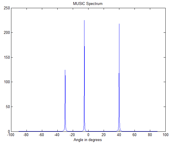
　　未做实数化处理，code:

clc;clear all;close all
%Ref:Narrowband direction of arrival estimation for antenna arrays
doas=[-30 -5 40]*pi/180; %DOA's of signals in rad.
P=[1 1 1]; %Power of incoming signals
N=10; %Number of array elements
K=1024; %Number of data snapshots
d=0.5; %Distance between elements in wavelengths
noise_var=1; %Variance of noise
r=length(doas); %Total number of signals
% Steering vector matrix. Columns will contain the steering vectors
% of the r signals
A=exp(-i*2*pi*d*(0:N-1)'*sin([doas(:).']));
% Signal and noise generation
sig=round(rand(r,K))*2-1; % Generate random BPSK symbols for each of the
% r signals
noise=sqrt(noise_var/2)*(randn(N,K)+i*randn(N,K)); %Uncorrelated noise
X=A*diag(sqrt(P))*sig+noise; %Generate data matrix
R=X*X'/K; %Spatial covariance matrix
[Q ,D]= svd(R); %Compute eigendecomposition of covariance matrix
[D,I]=sort(diag(D),1,'descend'); %Find r largest eigenvalues
Q=Q(:,I);%Sort?the?eigenvectors?to?put?signal?eigenvectors?first
Qs=Q (:,1:r); %Get the signal eigenvectors
Qn=Q(:,r+1:N); %Get the noise eigenvectors
% MUSIC algorithm
%?Define?angles?at?which?MUSIC???spectrum????will?be?computed
angles=(-90:0.1:90);
%Compute steering vectors corresponding values in angles
a1=exp(-i*2*pi*d*(0:N-1)'*sin([angles(:).']*pi/180));
for k=1:length(angles)%Compute?MUSIC???spectrum??
music_spectrum(k)= 1/(a1(:,k)'*Qn*Qn'*a1(:,k));
end
figure(1)
plot(angles,abs(music_spectrum))
title('MUSIC Spectrum')
xlabel('Angle in degrees')

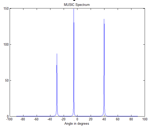
实数化处理，code：

clc;clear all;close all
%Ref:Narrowband direction of arrival estimation for antenna arrays
doas=[-30 -5 40]*pi/180; %DOA's of signals in rad.
P=[1 1 1]; %Power of incoming signals
N=10; %Number of array elements
K=1024; %Number of data snapshots
d=0.5; %Distance between elements in wavelengths
noise_var=1; %Variance of noise
r=length(doas); %Total number of signals
% Steering vector matrix. Columns will contain the steering vectors
% of the r signals
A=exp(-i*2*pi*d*(0:N-1)'*sin([doas(:).']));
% Signal and noise generation
sig=round(rand(r,K))*2-1; % Generate random BPSK symbols for each of the
% r signals
noise=sqrt(noise_var/2)*(randn(N,K)+i*randn(N,K)); %Uncorrelated noise
X=A*diag(sqrt(P))*sig+noise; %Generate data matrix
R=X*X'/K; %Spatial covariance matrix
%% Reconstruct
%实数
n = size(R);
I = eye(n/2);
J = fliplr(eye(n));
U = 1/sqrt(2)*[I fliplr(I);1j*fliplr(I) -1j*I];
R = 0.5*U*(R+J*conj(R)*J)*U';
% Reconstruct_end
[Q ,D]= svd(R); %Compute eigendecomposition of covariance matrix
[D,I]=sort(diag(D),1,'descend'); %Find r largest eigenvalues
Q=Q(:,I);%Sort?the?eigenvectors?to?put?signal?eigenvectors?first
Qs=Q (:,1:r); %Get the signal eigenvectors
Qn=Q(:,r+1:N); %Get the noise eigenvectors
% MUSIC algorithm
%?Define?angles?at?which?MUSIC???spectrum????will?be?computed
angles=(-90:0.1:90);
%Compute steering vectors corresponding values in angles
a1=exp(-i*2*pi*d*(0:N-1)'*sin([angles(:).']*pi/180));
for k=1:length(angles)%Compute?MUSIC???spectrum??
music_spectrum(k)= 1/(a1(:,k)'*U'*Qn*Qn'*U*a1(:,k));
end
figure(1)
plot(angles,abs(music_spectrum))
title('MUSIC Spectrum')
xlabel('Angle in degrees')