scikit-learning教程（二）统计学习科学数据处理的教程二

模型选择：选择估计量及其参数

得分和交叉验证的分数

如我们所看到的，每个估计者都会公开一种score可以判断新数据的拟合质量（或预测）的方法。越大越好。

>>>

>>> from sklearn import datasets, svm
>>> digits = datasets.load_digits()
>>> X_digits = digits.data
>>> y_digits = digits.target
>>> svc = svm.SVC(C=1, kernel='linear')
>>> svc.fit(X_digits[:-100], y_digits[:-100]).score(X_digits[-100:], y_digits[-100:])
0.97999999999999998

为了更好地测量预测精度（我们可以将其用作模型的拟合优势），我们可以连续地将数据分割成用于训练和测试的折叠：

>>>

>>> import numpy as np
>>> X_folds = np.array_split(X_digits, 3)
>>> y_folds = np.array_split(y_digits, 3)
>>> scores = list()
>>> for k in range(3):
...     # We use 'list' to copy, in order to 'pop' later on
...     X_train = list(X_folds)
...     X_test  = X_train.pop(k)
...     X_train = np.concatenate(X_train)
...     y_train = list(y_folds)
...     y_test  = y_train.pop(k)
...     y_train = np.concatenate(y_train)
...     scores.append(svc.fit(X_train, y_train).score(X_test, y_test))
>>> print(scores)
[0.93489148580968284, 0.95659432387312182, 0.93989983305509184]

这被称为KFold交叉验证。

交叉验证生成器

Scikit学习有一系列课程，可用于生成流行交叉验证策略的列车/测试指标列表。

它们公开了split一种接受要分割的输入数据集的方法，并为所选交叉验证策略的每次迭代产生列车/测试集合索引。

此示例显示了该split方法的示例用法。

>>>

>>> from sklearn.model_selection import KFold, cross_val_score
>>> X = ["a", "a", "b", "c", "c", "c"]
>>> k_fold = KFold(n_splits=3)
>>> for train_indices, test_indices in k_fold.split(X):
...      print('Train: %s | test: %s' % (train_indices, test_indices))
Train: [2 3 4 5] | test: [0 1]
Train: [0 1 4 5] | test: [2 3]
Train: [0 1 2 3] | test: [4 5]

然后可以轻松执行交叉验证：

>>>

>>> kfold = KFold(n_splits=3)
>>> [svc.fit(X_digits[train], y_digits[train]).score(X_digits[test], y_digits[test])
...          for train, test in k_fold.split(X_digits)]
[0.93489148580968284, 0.95659432387312182, 0.93989983305509184]

交叉验证分数可以使用cross_val_score助手直接计算 。给定估计器，交叉验证对象和输入数据集，cross_val_score将数据重复分为训练和测试集，使用训练集训练估计器，并根据每次交叉验证迭代的测试集计算得分。

默认情况下，使用估计器的score方法来计算单个分数。

参考指标模块，了解更多可用评分方法。

>>>

>>> cross_val_score(svc, X_digits, y_digits, cv=k_fold, n_jobs=-1)
array([ 0.93489149,  0.95659432,  0.93989983])

n_jobs = -1表示将在计算机的所有CPU上分派计算。

或者，scoring可以提供参数以指定替代评分方法。

>>>

>>> cross_val_score(svc, X_digits, y_digits, cv=k_fold,
...                 scoring='precision_macro')
array([ 0.93969761,  0.95911415,  0.94041254])

交叉验证生成器

KFold （n_splits，shuffle，random_state）	StratifiedKFold （n_iter，test_size，train_size，random_state）	GroupKFold （n_splits，shuffle，random_state）
将其分为K个折叠，K-1上的火车，然后在左侧测试。	与K-Fold相同，但保留每个折叠内的类分布。	确保同一组不在测试和训练集中。

ShuffleSplit （n_iter，test_size，train_size，random_state）	StratifiedShuffleSplit	GroupShuffleSplit
根据随机排列产生列车/测试指标。	与shuffle split相同，但保留了每次迭代中的类分布。	确保同一组不在测试和训练集中。

LeaveOneGroupOut （）	LeavePGroupsOut （p）的	LeaveOneOut （）
使用组数组来对观察进行分组。	离开P组。	留下一个观察。

LeavePOut （p）的	PredefinedSplit
留下P观察。	根据预定义的分割生成火车/测试指标。

行使

在数字数据集上，绘制SVC 具有线性内核的估计器的交叉验证分数作为参数的函数C（使用点对数网格，从1到10）。

import numpy as np
from sklearn.model_selection import cross_val_score
from sklearn import datasets, svm

digits = datasets.load_digits()
X = digits.data
y = digits.target

svc = svm.SVC(kernel='linear')
C_s = np.logspace(-10, 0, 10)

解决方案： 数字数据集练习的交叉验证

网格搜索和交叉验证的估计

网格搜索

scikit-learn提供了一个对象，给定的数据在参数网格中的估计器拟合期间计算分数，并选择参数以最大化交叉验证分数。该对象在构建期间使用估计器，并公开估计器API：

>>>

>>> from sklearn.model_selection import GridSearchCV, cross_val_score
>>> Cs = np.logspace(-6, -1, 10)
>>> clf = GridSearchCV(estimator=svc, param_grid=dict(C=Cs),
...                    n_jobs=-1)
>>> clf.fit(X_digits[:1000], y_digits[:1000])        
GridSearchCV(cv=None,...
>>> clf.best_score_                                  
0.925...
>>> clf.best_estimator_.C                            
0.0077...

>>> # Prediction performance on test set is not as good as on train set
>>> clf.score(X_digits[1000:], y_digits[1000:])      
0.943...

默认情况下，GridSearchCV使用三重交叉验证。然而，如果它检测到分类器被传递，而不是一个回归，它将使用分层3倍。

嵌套交叉验证

>>>

>>> cross_val_score(clf, X_digits, y_digits)
...                                               
array([ 0.938...,  0.963...,  0.944...])

并行执行两个交叉验证循环：一个通过 GridSearchCV估计器进行设置gamma，另一个通过 cross_val_score测量估计器的预测性能。得出的分数是对新数据的预测分数的无偏估计。

警告

 

您不能使用并行计算来嵌套对象（n_jobs不同于1）。

交叉验证的估计

可以在逐个算法的基础上更有效地进行交叉验证来设置参数。这就是为什么，对于某些估计，scikit学习公开交叉验证：评估通过交叉验证自动设置其参数的估计器性能估计器：

>>>

>>> from sklearn import linear_model, datasets
>>> lasso = linear_model.LassoCV()
>>> diabetes = datasets.load_diabetes()
>>> X_diabetes = diabetes.data
>>> y_diabetes = diabetes.target
>>> lasso.fit(X_diabetes, y_diabetes)
LassoCV(alphas=None, copy_X=True, cv=None, eps=0.001, fit_intercept=True,
    max_iter=1000, n_alphas=100, n_jobs=1, normalize=False, positive=False,
    precompute='auto', random_state=None, selection='cyclic', tol=0.0001,
    verbose=False)
>>> # The estimator chose automatically its lambda:
>>> lasso.alpha_ 
0.01229...

这些估计值被称为与其对应的类似，其名称附加“CV”。

行使

在糖尿病数据集上，找到最优正则化参数α。

奖金：您可以信赖多少选择阿尔法？

from sklearn import datasets
from sklearn.linear_model import LassoCV
from sklearn.linear_model import Lasso
from sklearn.model_selection import KFold
from sklearn.model_selection import cross_val_score

diabetes = datasets.load_diabetes()

解决方案： 糖尿病数据集练习的交叉验证

无监督学习：寻求数据表示

聚类：将观察分组在一起

问题在聚类中解决了

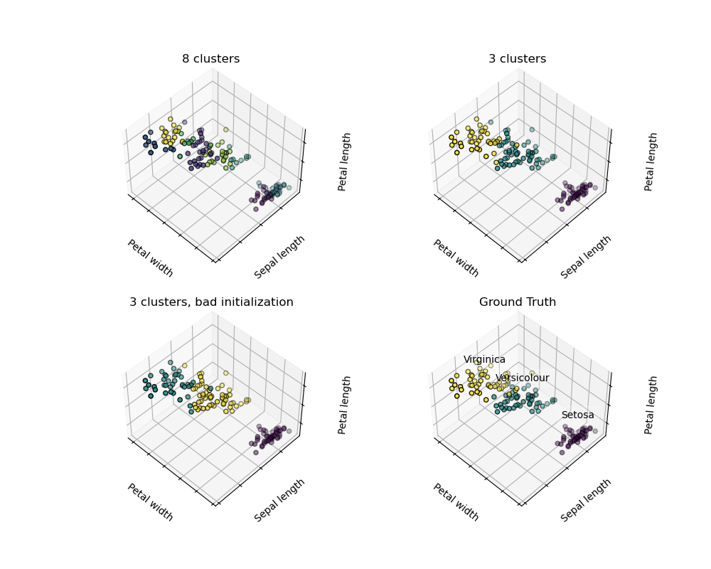
鉴于虹膜数据集，如果我们知道有3种类型的虹膜，但没有访问分类学家来标注它们：我们可以尝试一个 聚类任务：将观察结果分成称为聚类的完全分离的组。

K-means聚类

请注意，存在很多不同的聚类标准和相关算法。最简单的聚类算法是 K-means。

>>>

>>> from sklearn import cluster, datasets
>>> iris = datasets.load_iris()
>>> X_iris = iris.data
>>> y_iris = iris.target

>>> k_means = cluster.KMeans(n_clusters=3)
>>> k_means.fit(X_iris) 
KMeans(algorithm='auto', copy_x=True, init='k-means++', ...
>>> print(k_means.labels_[::10])
[1 1 1 1 1 0 0 0 0 0 2 2 2 2 2]
>>> print(y_iris[::10])
[0 0 0 0 0 1 1 1 1 1 2 2 2 2 2]

警告

 

绝对没有保证恢复地面真相。首先，选择正确的簇数很难。第二，该算法对初始化敏感，并且可以落入局部最小值，尽管scikit学习采用了几种技巧来缓解这个问题。

初始化不好	8个群集	地面事实

不要过度解释聚类结果

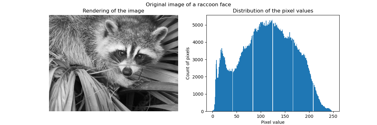
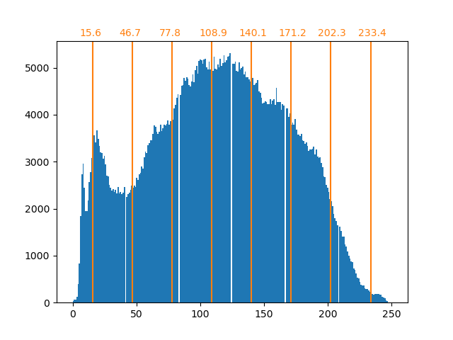
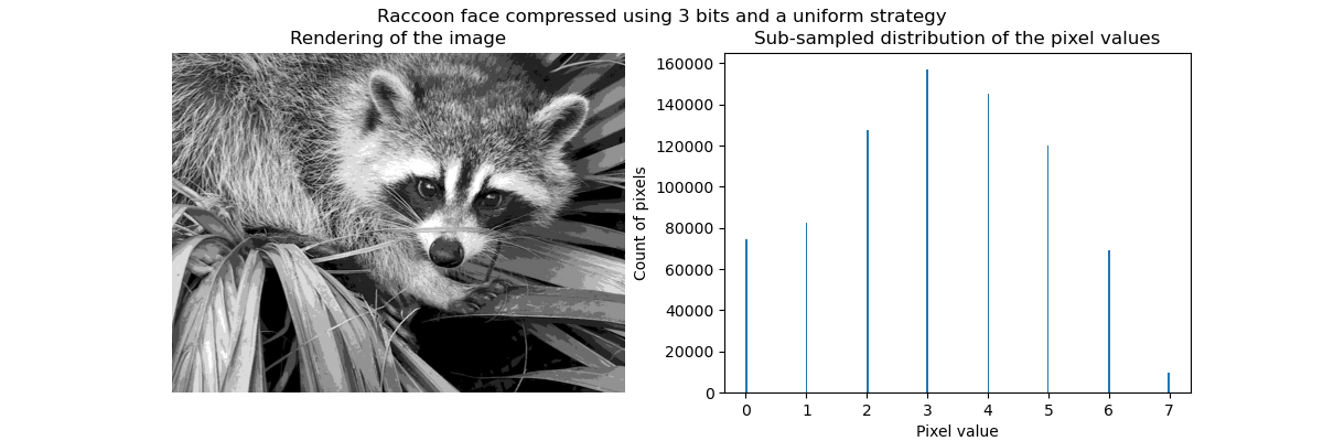
应用实例：矢量量化

特别是集体聚焦和KMeans可以被看作是选择少量样本来压缩信息的一种方式。这个问题有时被称为 矢量量化。例如，这可以用于对图像进行后缀：

>>>

>>> import scipy as sp
>>> try:
...    face = sp.face(gray=True)
... except AttributeError:
...    from scipy import misc
...    face = misc.face(gray=True)
>>> X = face.reshape((-1, 1)) # We need an (n_sample, n_feature) array
>>> k_means = cluster.KMeans(n_clusters=5, n_init=1)
>>> k_means.fit(X) 
KMeans(algorithm='auto', copy_x=True, init='k-means++', ...
>>> values = k_means.cluster_centers_.squeeze()
>>> labels = k_means.labels_
>>> face_compressed = np.choose(labels, values)
>>> face_compressed.shape = face.shape

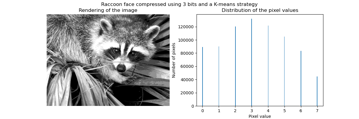原始图像	K均值量化	平仓	图像直方图

层次聚集：

甲分级聚类方法是一种类型的聚类分析的，其目的是建立聚类的层次结构。一般来说，这种技术的各种方法是：

• 集聚 - 自下而上的方法：每个观察在自己的集群中开始，集群被迭代地合并，以最小化连接标准。当感兴趣的集团仅由少数观察结果组成时，这种方法特别有意义。当簇的数量较大时，其计算效率要高于k-means。
• 分歧 - 自上而下的方法：所有的观察开始于一个群集，当层次结构向下移动时，迭代分裂。为了估计大量的群集，这种方法既缓慢（由于所有的观察开始于一个群集，它被递归地分解）和统计学上不合适。

连通约束聚类

通过聚集聚类，可以通过给出连通性图来指定哪些样本可以聚集在一起。scikit中的图表由它们的邻接矩阵表示。通常使用稀疏矩阵。这可以是有用的，例如，在聚类图像时检索连接的区域（有时也称为连接的组件）：

import matplotlib.pyplot as plt

from sklearn.feature_extraction.image import grid_to_graph
from sklearn.cluster import AgglomerativeClustering
from sklearn.utils.testing import SkipTest
from sklearn.utils.fixes import sp_version

if sp_version < (0, 12):
    raise SkipTest("Skipping because SciPy version earlier than 0.12.0 and "
                   "thus does not include the scipy.misc.face() image.")


###############################################################################
# Generate data
try:
    face = sp.face(gray=True)
except AttributeError:
    # Newer versions of scipy have face in misc
    from scipy import misc
    face = misc.face(gray=True)

# Resize it to 10% of the original size to speed up the processing
face = sp.misc.imresize(face, 0.10) / 255.

特征聚集

我们已经看到，稀疏性可以用来减轻维度的诅咒，即与特征数量相比，观察量不足。另一种方法是将类似特征合并在一起：特征聚集。这种方法可以通过在特征方向上聚类来实现，换句话说，聚类转置的数据。

>>>

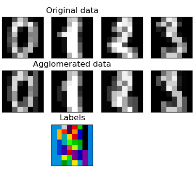
>>> digits = datasets.load_digits()
>>> images = digits.images
>>> X = np.reshape(images, (len(images), -1))
>>> connectivity = grid_to_graph(*images[0].shape)

>>> agglo = cluster.FeatureAgglomeration(connectivity=connectivity,
...                                      n_clusters=32)
>>> agglo.fit(X) 
FeatureAgglomeration(affinity='euclidean', compute_full_tree='auto',...
>>> X_reduced = agglo.transform(X)

>>> X_approx = agglo.inverse_transform(X_reduced)
>>> images_approx = np.reshape(X_approx, images.shape)

transform和inverse_transform方法

一些估计者会公开一种transform方法，例如降低数据集的维度。

分解：从信号到组件和加载

组件和装载

如果X是我们的多变量数据，那么我们要解决的问题是在不同的观察基础上重写：我们要学习加载L和一组组件C，使得X = LC。存在不同的标准来选择组件

主成分分析：

主分量分析（PCA）选择说明信号最大方差的连续分量。

 

上述观察点的点云在一个方向上是非常平坦的：三个单变量特征之一几乎可以使用另外两个方法精确计算。PCA查找数据不平坦的方向

用于变换数据时，PCA可以通过在主子空间上投影来降低数据的维数。

>>>

>>> # Create a signal with only 2 useful dimensions
>>> x1 = np.random.normal(size=100)
>>> x2 = np.random.normal(size=100)
>>> x3 = x1 + x2
>>> X = np.c_[x1, x2, x3]

>>> from sklearn import decomposition
>>> pca = decomposition.PCA()
>>> pca.fit(X)
PCA(copy=True, iterated_power='auto', n_components=None, random_state=None,
  svd_solver='auto', tol=0.0, whiten=False)
>>> print(pca.explained_variance_)  
[  2.18565811e+00   1.19346747e+00   8.43026679e-32]

>>> # As we can see, only the 2 first components are useful
>>> pca.n_components = 2
>>> X_reduced = pca.fit_transform(X)
>>> X_reduced.shape
(100, 2)

独立成分分析：

独立组件分析（ICA）选择组件，使其负载的分布具有最大量的独立信息。它能够恢复 非高斯独立信号：

>>>

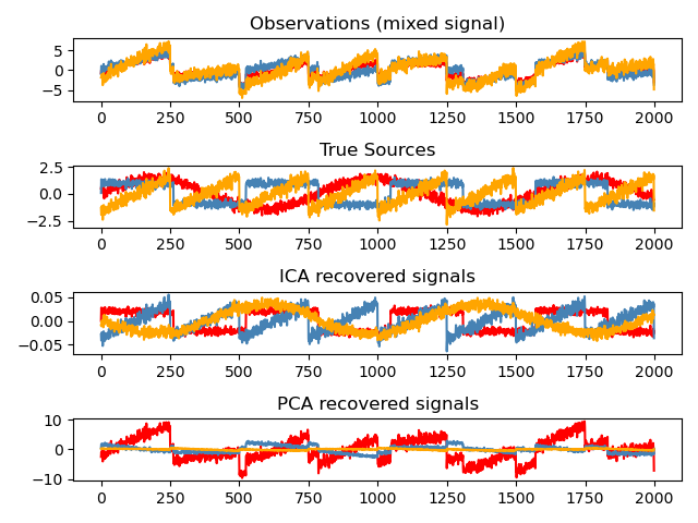
>>> # Generate sample data
>>> time = np.linspace(0, 10, 2000)
>>> s1 = np.sin(2 * time)  # Signal 1 : sinusoidal signal
>>> s2 = np.sign(np.sin(3 * time))  # Signal 2 : square signal
>>> S = np.c_[s1, s2]
>>> S += 0.2 * np.random.normal(size=S.shape)  # Add noise
>>> S /= S.std(axis=0)  # Standardize data
>>> # Mix data
>>> A = np.array([[1, 1], [0.5, 2]])  # Mixing matrix
>>> X = np.dot(S, A.T)  # Generate observations

>>> # Compute ICA
>>> ica = decomposition.FastICA()
>>> S_ = ica.fit_transform(X)  # Get the estimated sources
>>> A_ = ica.mixing_.T
>>> np.allclose(X,  np.dot(S_, A_) + ica.mean_)
True

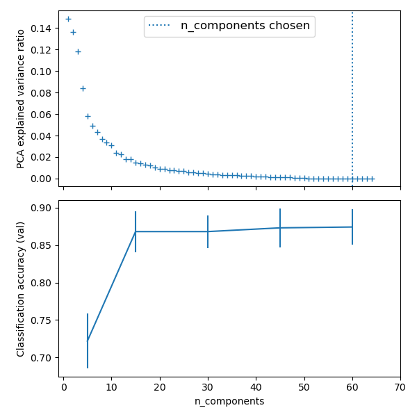
把它放在一起

流水

我们已经看到一些估计器可以转换数据，一些估计器可以预测变量。我们还可以创建组合估计：

from sklearn import linear_model, decomposition, datasets
from sklearn.pipeline import Pipeline
from sklearn.model_selection import GridSearchCV

logistic = linear_model.LogisticRegression()

pca = decomposition.PCA()
pipe = Pipeline(steps=[('pca', pca), ('logistic', logistic)])

digits = datasets.load_digits()
X_digits = digits.data
y_digits = digits.target

###############################################################################
# Plot the PCA spectrum
pca.fit(X_digits)

plt.figure(1, figsize=(4, 3))
plt.clf()
plt.axes([.2, .2, .7, .7])
plt.plot(pca.explained_variance_, linewidth=2)
plt.axis('tight')
plt.xlabel('n_components')
plt.ylabel('explained_variance_')

###############################################################################
# Prediction

n_components = [20, 40, 64]
Cs = np.logspace(-4, 4, 3)

#Parameters of pipelines can be set using ‘__’ separated parameter names:

estimator = GridSearchCV(pipe,
                         dict(pca__n_components=n_components,
                              logistic__C=Cs))
estimator.fit(X_digits, y_digits)

plt.axvline(estimator.best_estimator_.named_steps['pca'].n_components,
            linestyle=':', label='n_components chosen')
plt.legend(prop=dict(size=12))

使用特征面部识别

本例中使用的数据集是“野外标签面”的预处理摘录，也称为LFW：

http://vis-www.cs.umass.edu/lfw/lfw-funneled.tgz（233MB）

“”“ 
============================================= ==== 
使用特征面和SVM的面孔识别示例
=================================== ============

本示例中使用的数据集是
“野外标记的面孔” 的预处理摘录，也称为LFW_：

  http://vis-www.cs.umass.edu/lfw/lfw-funneled.tgz（233MB）

.. _LFW：http://vis-www.cs.umass.edu/lfw/

数据集中最有代表人数的5个预期结果：

================== ============ ======= ========== === ==== 
                   精度回忆f1分数支持
================== ============ ======= === ======= ======= 
     Ariel Sharon 0.67 0.92 0.77 13 
     Colin Powell 0.75 0.78 0.76 60 
  Donald Rumsfeld 0.78 0.67 0.72 27 
    George W Bush 0.86 0.86 0.86 146 
Gerhard Schroeder 0.76 0.76 0.76 25 
      Hugo Chavez 0.67 0.67 0.67 15 
       托尼·布莱尔0.81 0.69 0.75 36

      平均/合计0.80 0.80 0.80 322 
================== ============ ======= ==== ==== =======

from __future__ import print_function

from time import time
import logging
import matplotlib.pyplot as plt

from sklearn.model_selection import train_test_split
from sklearn.model_selection import GridSearchCV
from sklearn.datasets import fetch_lfw_people
from sklearn.metrics import classification_report
from sklearn.metrics import confusion_matrix
from sklearn.decomposition import PCA
from sklearn.svm import SVC


print(__doc__)

# Display progress logs on stdout
logging.basicConfig(level=logging.INFO, format='%(asctime)s%(message)s')


###############################################################################
# Download the data, if not already on disk and load it as numpy arrays

lfw_people = fetch_lfw_people(min_faces_per_person=70, resize=0.4)

# introspect the images arrays to find the shapes (for plotting)
n_samples, h, w = lfw_people.images.shape

# for machine learning we use the 2 data directly (as relative pixel
# positions info is ignored by this model)
X = lfw_people.data
n_features = X.shape[1]

# the label to predict is the id of the person
y = lfw_people.target
target_names = lfw_people.target_names
n_classes = target_names.shape[0]

print("Total dataset size:")
print("n_samples: %d" % n_samples)
print("n_features: %d" % n_features)
print("n_classes: %d" % n_classes)


###############################################################################
# Split into a training set and a test set using a stratified k fold

# split into a training and testing set
X_train, X_test, y_train, y_test = train_test_split(
    X, y, test_size=0.25, random_state=42)


###############################################################################
# Compute a PCA (eigenfaces) on the face dataset (treated as unlabeled
# dataset): unsupervised feature extraction / dimensionality reduction
n_components = 150

print("Extracting the top %d eigenfaces from %d faces"
      % (n_components, X_train.shape[0]))
t0 = time()
pca = PCA(n_components=n_components, svd_solver='randomized',
          whiten=True).fit(X_train)
print("done in %0.3fs" % (time() - t0))

eigenfaces = pca.components_.reshape((n_components, h, w))

print("Projecting the input data on the eigenfaces orthonormal basis")
t0 = time()
X_train_pca = pca.transform(X_train)
X_test_pca = pca.transform(X_test)
print("done in %0.3fs" % (time() - t0))


###############################################################################
# Train a SVM classification model

print("Fitting the classifier to the training set")
t0 = time()
param_grid = {'C': [1e3, 5e3, 1e4, 5e4, 1e5],
              'gamma': [0.0001, 0.0005, 0.001, 0.005, 0.01, 0.1], }
clf = GridSearchCV(SVC(kernel='rbf', class_weight='balanced'), param_grid)
clf = clf.fit(X_train_pca, y_train)
print("done in %0.3fs" % (time() - t0))
print("Best estimator found by grid search:")
print(clf.best_estimator_)


###############################################################################
# Quantitative evaluation of the model quality on the test set

print("Predicting people's names on the test set")
t0 = time()
y_pred = clf.predict(X_test_pca)
print("done in %0.3fs" % (time() - t0))

print(classification_report(y_test, y_pred, target_names=target_names))
print(confusion_matrix(y_test, y_pred, labels=range(n_classes)))


###############################################################################
# Qualitative evaluation of the predictions using matplotlib

def plot_gallery(images, titles, h, w, n_row=3, n_col=4):
    """Helper function to plot a gallery of portraits"""
    plt.figure(figsize=(1.8 * n_col, 2.4 * n_row))
    plt.subplots_adjust(bottom=0, left=.01, right=.99, top=.90, hspace=.35)
    for i in range(n_row * n_col):
        plt.subplot(n_row, n_col, i + 1)
        plt.imshow(images[i].reshape((h, w)), cmap=plt.cm.gray)
        plt.title(titles[i], size=12)
        plt.xticks(())
        plt.yticks(())


# plot the result of the prediction on a portion of the test set

def title(y_pred, y_test, target_names, i):
    pred_name = target_names[y_pred[i]].rsplit(' ', 1)[-1]
    true_name = target_names[y_test[i]].rsplit(' ', 1)[-1]
    return 'predicted: %s\ntrue:      %s' % (pred_name, true_name)

prediction_titles = [title(y_pred, y_test, target_names, i)
                     for i in range(y_pred.shape[0])]

plot_gallery(X_test, prediction_titles, h, w)

# plot the gallery of the most significative eigenfaces

eigenface_titles = ["eigenface %d" % i for i in range(eigenfaces.shape[0])]
plot_gallery(eigenfaces, eigenface_titles, h, w)

plt.show()

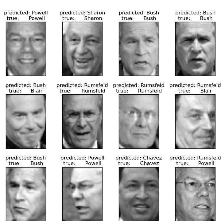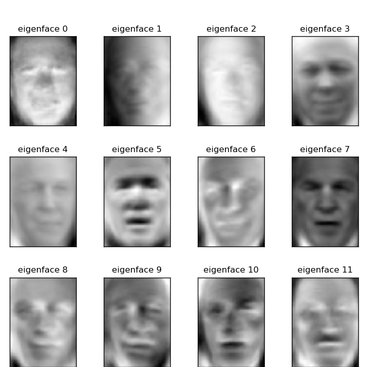预测	特征脸

数据集中最有代表人数的5个预期结果：

                   精准    回忆  f1 - 得分   支持

Gerhard_Schroeder        0.91       0.75       0.82         28 
  Donald_Rumsfeld        0.84       0.82       0.83         33 
       Tony_Blair        0.65       0.82       0.73         34 
     Colin_Powell        0.78       0.88       0.83         58 
    George_W_Bush        0.93       0.86       0.90        129

      平均 /  总计       0.86       0.84       0.85        282

开放式问题：证券市场结构

我们可以预测Google在特定时间段内的股价变动吗？

学习图形结构

模型选择：选择估计量及其参数

得分和交叉验证的分数

如我们所看到的，每个估计者都会公开一种score可以判断新数据的拟合质量（或预测）的方法。越大越好。

>>>

>>> 从 sklearn  导入 数据集， svm 
>>> digits  =  数据集。load_digits （）
>>> X_digits  =  数字。数据
>>> y_digits  =  数字。目标
>>> svc  =  svm 。SVC （C = 1 ， kernel = 'linear' ）
>>> svc 。fit （X_digits [：- 100 ]， y_digits [：- 100 ]）。得分（X_digits [ - 100 ：]， y_digits [ - 100 ：]）
0.97999999999999998

为了更好地测量预测精度（我们可以将其用作模型的拟合优势），我们可以连续地将数据分割成用于训练和测试的折叠：

>>>

>>> 将 numpy  作为 np 
>>> X_folds  =  np 。array_split （X_digits ， 3 ）
>>> y_folds  =  np 。array_split （y_digits ， 3 ）
>>> scores  =  list （）
>>> for  k  in  range （3 ）：
...     ＃我们使用'list'复制，以便稍后在“pop” 
...     X_train  =  列表（X_folds ）
..     。X_test   =  X_train 。pop （k ）
...     X_train  =  np 。连接（X_train ）
...     y_train  =  list （y_folds ）
...     y_test   =  y_train 。pop （k ）
...     y_train  =  np 。连接（y_train ）
...     得分。追加（SVC 。适合（X_train ， y_train ）。分数（X_test ， y_test ））
>>> print （scores ）
[0.93489148580968284，0.95659432387312182，0.93989983305509184]

这被称为KFold交叉验证。

交叉验证生成器

Scikit学习有一系列课程，可用于生成流行交叉验证策略的列车/测试指标列表。

它们公开了split一种接受要分割的输入数据集的方法，并为所选交叉验证策略的每次迭代产生列车/测试集合索引。

此示例显示了该split方法的示例用法。

>>>

>>> 从 sklearn.model_selection  导入 KFold ， cross_val_score 
>>> X  =  [ “a” ， “a” ， “b” ， “c” ， “c” ， “c” ] 
>>> k_fold  =  KFold （n_splits = 3 ）
>>> for  train_indices ， test_indices  in  k_fold 。split （X ）：
...      print （'Train：％s | 测试：％s '  ％ （train_indices ， test_indices ））
火车：[2 3 4 5] | 测试：[0 1] 
火车：[0 1 4 5] | 测试：[2 3] 
火车：[0 1 2 3] | 测试：[4 5]

然后可以轻松执行交叉验证：

>>>

>>> kfold  =  KFold （n_splits = 3 ）
>>> [ svc 。fit （X_digits [ train ]， y_digits [ train ]）。得分（X_digits [ test ]， y_digits [ test ]）
...          用于 列车， 以k_fold 测试 。split （X_digits ）] [0.93489148580968284，0.95659432387312182，0.93989983305509184] 

交叉验证分数可以使用cross_val_score助手直接计算 。给定估计器，交叉验证对象和输入数据集，cross_val_score将数据重复分为训练和测试集，使用训练集训练估计器，并根据每次交叉验证迭代的测试集计算得分。

默认情况下，使用估计器的score方法来计算单个分数。

参考指标模块，了解更多可用评分方法。

>>>

>>> cross_val_score （svc ， X_digits ， y_digits ， cv = k_fold ， n_jobs =  - 1 ）
array（[0.93489149,0.95659432,0.93989983]）

n_jobs = -1表示将在计算机的所有CPU上分派计算。

或者，scoring可以提供参数以指定替代评分方法。

>>>

>>> cross_val_score （svc ， X_digits ， y_digits ， cv = k_fold ，
...                 scoring = 'precision_macro' ）
array（[0.93969761，0.95911415，0.94041254]）

交叉验证生成器

KFold （n_splits，shuffle，random_state）	StratifiedKFold （n_iter，test_size，train_size，random_state）	GroupKFold （n_splits，shuffle，random_state）
将其分为K个折叠，K-1上的火车，然后在左侧测试。	与K-Fold相同，但保留每个折叠内的类分布。	确保同一组不在测试和训练集中。

ShuffleSplit （n_iter，test_size，train_size，random_state）	StratifiedShuffleSplit	GroupShuffleSplit
根据随机排列产生列车/测试指标。	与shuffle split相同，但保留了每次迭代中的类分布。	确保同一组不在测试和训练集中。

LeaveOneGroupOut （）	LeavePGroupsOut （p）的	LeaveOneOut （）
使用组数组来对观察进行分组。	离开P组。	留下一个观察。

LeavePOut （p）的	PredefinedSplit
留下P观察。	根据预定义的分割生成火车/测试指标。

行使

在数字数据集上，绘制SVC 具有线性内核的估计器的交叉验证分数作为参数的函数C（使用点对数网格，从1到10）。

导入 numpy的 是 NP 
从 sklearn.model_selection  进口 cross_val_score 
从 sklearn  进口 数据集， SVM

digits  =  数据集。load_digits （）
X  =  数字。数据
y  =  数字。目标

svc  =  svm 。SVC （kernel = 'linear' ）
C_s  =  np 。LOGSPACE （- 10 ， 0 ， 10 ）

解决方案： 数字数据集练习的交叉验证

网格搜索和交叉验证的估计

网格搜索

scikit-learn提供了一个对象，给定的数据在参数网格中的估计器拟合期间计算分数，并选择参数以最大化交叉验证分数。该对象在构建期间使用估计器，并公开估计器API：

>>>

>>> 从 sklearn.model_selection  导入 GridSearchCV ， cross_val_score 
>>> Cs  =  np 。LOGSPACE （- 6 ， - 1 ， 10 ）
>>> CLF  =  GridSearchCV （估计= SVC ， param_grid = 字典（C ^ = 铯），
...                    n_jobs = - 1 ）
>>> CLF 。fit （X_digits [：1000 ]，         

                                  

                            


>>> ＃测试集上的预测性能不如火车上的设置
>>> clf 。得分（X_digits [ 1000 ：]， y_digits [ 1000 ：]）      
0.943 ...

默认情况下，GridSearchCV使用三重交叉验证。然而，如果它检测到分类器被传递，而不是一个回归，它将使用分层3倍。

嵌套交叉验证

>>>

>>> cross_val_score （clf ， X_digits ， y_digits ）
...                                               
array（[ 0.938 ...，0.963 ...，0.944 ...]）

并行执行两个交叉验证循环：一个通过 GridSearchCV估计器进行设置gamma，另一个通过 cross_val_score测量估计器的预测性能。得出的分数是对新数据的预测分数的无偏估计。

警告

 

您不能使用并行计算来嵌套对象（n_jobs不同于1）。

交叉验证的估计

可以在逐个算法的基础上更有效地进行交叉验证来设置参数。这就是为什么，对于某些估计，scikit学习公开交叉验证：评估通过交叉验证自动设置其参数的估计器性能估计器：

>>>

>>> 从 sklearn  import  linear_model ， datasets 
>>> lasso  =  linear_model 。LassoCV （）
>>> 糖尿病 =  数据集。load_diabetes （）
>>> X_diabetes  =  糖尿病。数据
>>> y_diabetes  =  糖尿病。目标
>>> 套索。fit （X_diabetes ， y_diabetes ）
LassoCV（alphas = None，copy_X = True，cv = None，eps = 0.001，fit_intercept = True，
    max_iter = 1000，n_alphas = 100，n_jobs = 1，normalize = False，positive = False，
    precompute ='auto'，random_state = None，selection ='cyclic'，tol = 0.0001，
    verbose = False）
>>> ＃自动选择其lambda：
>>> lasso 。alpha_  
0.01229 ...

这些估计值被称为与其对应的类似，其名称附加“CV”。

行使

在糖尿病数据集上，找到最优正则化参数α。

奖金：您可以信赖多少选择阿尔法？

从 sklearn  进口 数据集
从 sklearn.linear_model  进口 LassoCV 
从 sklearn.linear_model  进口 拉索
从 sklearn.model_selection  进口 KFold 
从 sklearn.model_selection  进口 cross_val_score

糖尿病 =  数据集。load_diabetes （）

解决方案： 糖尿病数据集练习的交叉验证