Deep learning：二十二(linear decoder练习)

 

　　前言：

　　本节是练习Linear decoder的应用，关于Linear decoder的相关知识介绍请参考：Deep learning：十七(Linear Decoders，Convolution和Pooling)，实验步骤参考Exercise: Implement deep networks for digit classification。本次实验是用linear decoder的sparse autoencoder来训练出stl-10数据库图片的patch特征。并且这次的训练权值是针对rgb图像块的。

 

　　基础知识：

　　PCA Whitening是保证数据各维度的方差为1，而ZCA Whitening是保证数据各维度的方差相等即可，不一定要唯一。并且这两种whitening的一般用途也不一样，PCA Whitening主要用于降维且去相关性，而ZCA Whitening主要用于去相关性，且尽量保持原数据。

　　Matlab的一些知识：

　　函数句柄的好处就是把一个函数作为参数传入到本函数中，在该函数内部可以利用该函数进行各种运算得出最后需要的结果，比如说函数中要用到各种求导求积分的方法，如果是传入该函数经过各种运算后的值的话，那么在调用该函数前就需要不少代码，这样比较累赘，所以采用函数句柄后这些代码直接放在了函数内部，每调用一次无需在函数外面实现那么多的东西。

　　Matlab中保存各种数据时可以采用save函数，并将其保持为.mat格式的，这样在matlab的current folder中看到的是.mat格式的文件，但是直接在文件夹下看，它是不直接显示后缀的，且显示的是Microsoft Access Table Shortcut，也就是.mat的简称。

　　关于实验的一些说明：

　　在Ng的教程和实验中，它的输入样本矩阵是每一列代表一个样本的，列数为样本的总个数。

　　matlab中矩阵64*10w大小肯定是可以的。

　　在本次实验中，ZCA Whitening是针对patches进行的，且patches的均值化是对每一维进行的（感觉这种均值化比较靠谱，前面有文章是进行对patch中一个样本求均值，感觉那样很不靠谱，不过那是在natural image中做的，因为natural image每一维的统计特性都一样，所以可以那样均值化，但还是感觉不太靠谱）。因为使用的是ZCA whitening，所以新的向量并没有进行降维，只是去了相关性和让每一维的方差都相等而已。另外，由此可见，在进行数据Whitening时并不需要对原始的大图片进行whitening，而是你用什么数据输入网络去训练就对什么数据进行whitening，而这里，是用的小patches来训练的，所以应该对小patches进行whitening。

　　关于本次实验的一些数据和变量分配如下：

　　总共需训练的样本矩阵大小为192*100000。因为输入训练的一个patch大小为8*8的，所以网络的输入层节点数为192（=8*8*3，因为是3通道的，每一列按照rgb的顺序排列），另外本次试验的隐含层个数为400，权值惩罚系数为0.003，稀疏性惩罚系数为5，稀疏性体现在3.5%的隐含层节点被激发。ZCA白化时分母加上0.1的值防止出现大的数值。

　　用的是Linear decoder，所以最后的输出层的激发函数为1，即输出和输入相等。这样在问题内部的计算量变小了点。

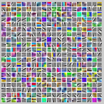
　　程序中最后需要把学习到的网络权值给显示出来，不过这个显示的内容已经包括了whitening部分了，所以是whitening和sparse autoencoder的组合。程序中显示用的是displayColorNetwork( (W*ZCAWhite)');

　　这里为什么要用(W*ZCAWhite)'呢？首先，使用W*ZCAWhite是因为每个样本x输入网络，其输出等价于W*ZCAWhite*x；另外，由于W*ZCAWhite的每一行才是一个隐含节点的变换值,而displayColorNetwork函数是把每一列显示一个小图像块的，所以需要对其转置。

 

　　实验结果：

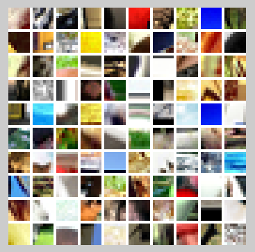
　　原始图片截图：

 　　

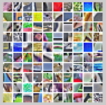
　　ZCA Whitening后截图;

 　　

　　学习到的400个特征显示如下：

 　　

 

　　实验主要部分代码：

%% CS294A/CS294W Linear Decoder Exercise

%  Instructions
%  ------------
% 
%  This file contains code that helps you get started on the
%  linear decoder exericse. For this exercise, you will only need to modify
%  the code in sparseAutoencoderLinearCost.m. You will not need to modify
%  any code in this file.

%%======================================================================
%% STEP 0: Initialization
%  Here we initialize some parameters used for the exercise.

imageChannels = 3;     % number of channels (rgb, so 3)

patchDim   = 8;          % patch dimension
numPatches = 100000;   % number of patches

visibleSize = patchDim * patchDim * imageChannels;  % number of input units 
outputSize  = visibleSize;   % number of output units
hiddenSize  = 400;           % number of hidden units %中间的隐含层还变多了

sparsityParam = 0.035; % desired average activation of the hidden units.
lambda = 3e-3;         % weight decay parameter       
beta = 5;              % weight of sparsity penalty term       

epsilon = 0.1;           % epsilon for ZCA whitening

%%======================================================================
%% STEP 1: Create and modify sparseAutoencoderLinearCost.m to use a linear decoder,
%          and check gradients
%  You should copy sparseAutoencoderCost.m from your earlier exercise 
%  and rename it to sparseAutoencoderLinearCost.m. 
%  Then you need to rename the function from sparseAutoencoderCost to
%  sparseAutoencoderLinearCost, and modify it so that the sparse autoencoder
%  uses a linear decoder instead. Once that is done, you should check 
% your gradients to verify that they are correct.

% NOTE: Modify sparseAutoencoderCost first!

% To speed up gradient checking, we will use a reduced network and some
% dummy patches

debugHiddenSize = 5;
debugvisibleSize = 8;
patches = rand([8 10]);%随机产生10个样本，每个样本为一个8维的列向量，元素值为0~1
theta = initializeParameters(debugHiddenSize, debugvisibleSize); 

[cost, grad] = sparseAutoencoderLinearCost(theta, debugvisibleSize, debugHiddenSize, ...
                                           lambda, sparsityParam, beta, ...
                                           patches);

% Check gradients
numGrad = computeNumericalGradient( @(x) sparseAutoencoderLinearCost(x, debugvisibleSize, debugHiddenSize, ...
                                                  lambda, sparsityParam, beta, ...
                                                  patches), theta);

% Use this to visually compare the gradients side by side
disp([numGrad cost]); 

diff = norm(numGrad-grad)/norm(numGrad+grad);
% Should be small. In our implementation, these values are usually less than 1e-9.
disp(diff); 

assert(diff < 1e-9, 'Difference too large. Check your gradient computation again');

% NOTE: Once your gradients check out, you should run step 0 again to
%       reinitialize the parameters
%}

%%======================================================================
%% STEP 2: Learn features on small patches
%  In this step, you will use your sparse autoencoder (which now uses a 
%  linear decoder) to learn features on small patches sampled from related
%  images.

%% STEP 2a: Load patches
%  In this step, we load 100k patches sampled from the STL10 dataset and
%  visualize them. Note that these patches have been scaled to [0,1]

load stlSampledPatches.mat

displayColorNetwork(patches(:, 1:100));

%% STEP 2b: Apply preprocessing
%  In this sub-step, we preprocess the sampled patches, in particular, 
%  ZCA whitening them. 
% 
%  In a later exercise on convolution and pooling, you will need to replicate 
%  exactly the preprocessing steps you apply to these patches before 
%  using the autoencoder to learn features on them. Hence, we will save the
%  ZCA whitening and mean image matrices together with the learned features
%  later on.

% Subtract mean patch (hence zeroing the mean of the patches)
meanPatch = mean(patches, 2);  %注意这里减掉的是每一维属性的均值，为什么会和其它的不同呢？
patches = bsxfun(@minus, patches, meanPatch);%每一维都均值化

% Apply ZCA whitening
sigma = patches * patches' / numPatches;
[u, s, v] = svd(sigma);
ZCAWhite = u * diag(1 ./ sqrt(diag(s) + epsilon)) * u';%求出ZCAWhitening矩阵
patches = ZCAWhite * patches;
figure
displayColorNetwork(patches(:, 1:100));

%% STEP 2c: Learn features
%  You will now use your sparse autoencoder (with linear decoder) to learn
%  features on the preprocessed patches. This should take around 45 minutes.

theta = initializeParameters(hiddenSize, visibleSize);

% Use minFunc to minimize the function
addpath minFunc/

options = struct;
options.Method = 'lbfgs'; 
options.maxIter = 400;
options.display = 'on';

[optTheta, cost] = minFunc( @(p) sparseAutoencoderLinearCost(p, ...
                                   visibleSize, hiddenSize, ...
                                   lambda, sparsityParam, ...
                                   beta, patches), ...
                              theta, options);%注意它的参数

% Save the learned features and the preprocessing matrices for use in 
% the later exercise on convolution and pooling
fprintf('Saving learned features and preprocessing matrices...\n');                          
save('STL10Features.mat', 'optTheta', 'ZCAWhite', 'meanPatch');
fprintf('Saved\n');

%% STEP 2d: Visualize learned features

W = reshape(optTheta(1:visibleSize * hiddenSize), hiddenSize, visibleSize);
b = optTheta(2*hiddenSize*visibleSize+1:2*hiddenSize*visibleSize+hiddenSize);
figure;
%这里为什么要用(W*ZCAWhite)'呢？首先，使用W*ZCAWhite是因为每个样本x输入网络，
%其输出等价于W*ZCAWhite*x；另外，由于W*ZCAWhite的每一行才是一个隐含节点的变换值
%而displayColorNetwork函数是把每一列显示一个小图像块的，所以需要对其转置。
displayColorNetwork( (W*ZCAWhite)');

 

 sparseAutoencoderLinearCost.m:

function [cost,grad] = sparseAutoencoderLinearCost(theta, visibleSize, hiddenSize, ...
                                                            lambda, sparsityParam, beta, data)
% -------------------- YOUR CODE HERE --------------------
% Instructions:
%   Copy sparseAutoencoderCost in sparseAutoencoderCost.m from your
%   earlier exercise onto this file, renaming the function to
%   sparseAutoencoderLinearCost, and changing the autoencoder to use a
%   linear decoder.
% -------------------- YOUR CODE HERE --------------------                                    
% The input theta is a vector because minFunc only deal with vectors. In
% this step, we will convert theta to matrix format such that they follow
% the notation in the lecture notes.
W1 = reshape(theta(1:hiddenSize*visibleSize), hiddenSize, visibleSize);
W2 = reshape(theta(hiddenSize*visibleSize+1:2*hiddenSize*visibleSize), visibleSize, hiddenSize);
b1 = theta(2*hiddenSize*visibleSize+1:2*hiddenSize*visibleSize+hiddenSize);
b2 = theta(2*hiddenSize*visibleSize+hiddenSize+1:end);

% Loss and gradient variables (your code needs to compute these values)
m = size(data, 2);%样本点的个数

%% ---------- YOUR CODE HERE --------------------------------------
%  Instructions: Compute the loss for the Sparse Autoencoder and gradients
%                W1grad, W2grad, b1grad, b2grad
%
%  Hint: 1) data(:,i) is the i-th example
%        2) your computation of loss and gradients should match the size
%        above for loss, W1grad, W2grad, b1grad, b2grad

% z2 = W1 * x + b1
% a2 = f(z2)
% z3 = W2 * a2 + b2
% h_Wb = a3 = f(z3)

z2 = W1 * data + repmat(b1, [1, m]);
a2 = sigmoid(z2);
z3 = W2 * a2 + repmat(b2, [1, m]);
a3 = z3;

rhohats = mean(a2,2);
rho = sparsityParam;
KLsum = sum(rho * log(rho ./ rhohats) + (1-rho) * log((1-rho) ./ (1-rhohats)));


squares = (a3 - data).^2;
squared_err_J = (1/2) * (1/m) * sum(squares(:));
weight_decay_J = (lambda/2) * (sum(W1(:).^2) + sum(W2(:).^2));
sparsity_J = beta * KLsum;

cost = squared_err_J + weight_decay_J + sparsity_J;%损失函数值

% delta3 = -(data - a3) .* fprime(z3);
% but fprime(z3) = a3 * (1-a3)
delta3 = -(data - a3);
beta_term = beta * (- rho ./ rhohats + (1-rho) ./ (1-rhohats));
delta2 = ((W2' * delta3) + repmat(beta_term, [1,m]) ) .* a2 .* (1-a2);

W2grad = (1/m) * delta3 * a2' + lambda * W2;
b2grad = (1/m) * sum(delta3, 2);
W1grad = (1/m) * delta2 * data' + lambda * W1;
b1grad = (1/m) * sum(delta2, 2);

%-------------------------------------------------------------------
% Convert weights and bias gradients to a compressed form
% This step will concatenate and flatten all your gradients to a vector
% which can be used in the optimization method.
grad = [W1grad(:) ; W2grad(:) ; b1grad(:) ; b2grad(:)];

end
%-------------------------------------------------------------------
% We are giving you the sigmoid function, you may find this function
% useful in your computation of the loss and the gradients.
function sigm = sigmoid(x)

    sigm = 1 ./ (1 + exp(-x));
end

 

　　参考资料：

     Deep learning：十七(Linear Decoders，Convolution和Pooling)

     Exercise: Implement deep networks for digit classification