Standard deviation

Posted on 2007-07-31 16:28 sunrack 阅读(1765) 评论(2) 编辑收藏举报

Standard deviation

From Wikipedia, the free encyclopedia

In probability and statistics, the standard deviation of a probability distribution, random variable, or population or multiset of values is a measure of the spread of its values. It is usually denoted with the letter σ (lower case sigma). It is defined as the square root of the variance.

To understand standard deviation, keep in mind that variance is the average of the squared differences between data points and the mean. Variance is tabulated in units squared. Standard deviation, being the square root of that quantity, therefore measures the spread of data about the mean, measured in the same units as the data.

Said more formally, the standard deviation is the root mean square (RMS) deviation of values from their arithmetic mean.

For example, in the population {4, 8}, the mean is 6 and the deviations from mean are {-2, 2}. Those deviations squared are {4, 4} the average of which (the variance) is 4. Therefore, the standard deviation is 2. In this case 100% of the values in the population are at one standard deviation of the mean.

The standard deviation is the most common measure of statistical dispersion, measuring how widely spread the values in a data set are. If the data points are close to the mean, then the standard deviation is small. As well, if many data points are far from the mean, then the standard deviation is large. If all the data values are equal, then the standard deviation is zero.

For a population, the standard deviation can be estimated by a modified standard deviation (s) of a sample. The formulae are given below.

[hide]

[edit] Definition and calculation

[edit] Standard deviation of a random variable

The standard deviation of a random variable X is defined as:

$\sigma = \sqrt{\operatorname{E}((X-\operatorname{E}(X))^2)}$ $= \sqrt{\operatorname{E}(X^2) - (\operatorname{E}(X))^2}$

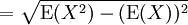
where E(X) is the expected value of X.

Not all random variables have a standard deviation, since these expected values need not exist. For example, the standard deviation of a random variable which follows a Cauchy distribution is undefined.

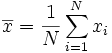
If the random variable X takes on the values $x_1,\cdots,x_N$ (which are real numbers) with equal probability, then its standard deviation can be computed as follows. First, the mean of X, $\overline{x}$ , is defined as a summation:

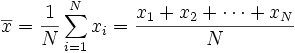
$\overline{x} = \frac{1}{N}\sum_{i=1}^N x_i = \frac{x_1+x_2+\cdots+x_N}{N}$

where N is the number of samples taken. Next, the standard deviation simplifies to

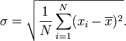
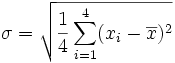
$\sigma = \sqrt{\frac{1}{N} \sum_{i=1}^N (x_i - \overline{x})^2}.$

In other words, the standard deviation of a discrete uniform random variable X can be calculated as follows:

For each value $x i$ calculate the difference $x_i - \overline{x}$ between $x i$ and the average value $\overline{x}$ .
Calculate the squares of these differences.
Find the average of the squared differences. This quantity is the variance $σ 2$ .
Take the square root of the variance.

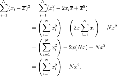
The above expression can also be replaced with

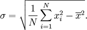
$\sigma = \sqrt{\frac{1}{N} \sum_{i=1}^N x_i^2 - \overline{x}^2}.$

Equality of these two expressions can be shown by a bit of algebra:

$\begin{align} \sum_{i=1}^N (x_i - \overline{x})^2 & = {} \sum_{i=1}^N (x_i^2 - 2 x_i\overline{x} + \overline{x}^2) \\ & {} = \left(\sum_{i=1}^N x_i^2\right) - \left(2 \overline{x} \sum_{i=1}^N x_i\right) + N\overline{x}^2 \\ & {} = \left(\sum_{i=1}^N x_i^2\right) - 2 \overline{x} (N\overline{x}) + N\overline{x}^2 \\ & {} = \left(\sum_{i=1}^N x_i^2\right) - N\overline{x}^2. \end{align}$

[edit] Estimating population standard deviation from sample standard deviation

In the real world, finding the standard deviation of an entire population is unrealistic except in certain cases, such as standardized testing, where every member of a population is sampled. In most cases, the standard deviation is estimated by examining a random sample taken from the population. The most common measure used is the sample standard deviation, which is defined by

$s = \sqrt{\frac{1}{N-1} \sum_{i=1}^N (x_i - \overline{x})^2}\,,$

where $\scriptstyle\{x_1,\,x_2,\,\ldots,\,x_N\}$ is the sample and $\scriptstyle\overline{x}$ is the mean of the sample. The denominator N − 1 is the number of degrees of freedom in the vector $\scriptstyle(x_1-\overline{x},\,\dots,\,x_N-\overline{x})$ .

The reason for this definition is that s² is an unbiased estimator for the variance σ² of the underlying population, if that variance exists and the sample values are drawn independently with replacement. However, s is not an unbiased estimator for the standard deviation σ; it tends to underestimate the population standard deviation. Although an unbiased estimator for σ is known when the random variable is normally distributed, the formula is complicated and amounts to a minor correction. Moreover, unbiasedness, in this sense of the word, is not always desirable; see bias of an estimator.

Another estimator sometimes used is the similar expression

$\sqrt{\frac{1}{N} \sum_{i=1}^N (x_i - \overline{x})^2}\,\,.$

This form has a uniformly smaller mean squared error than does the unbiased estimator, and is the maximum-likelihood estimate when the population is normally distributed.

[edit] Example

We will show how to calculate the standard deviation of a population. Our example will use the ages of four young children: { 5, 6, 8, 9 }.

Step 1. Calculate the mean average, $\overline{x}$ :

$\overline{x}=\frac{1}{N}\sum_{i=1}^N x_i$

We have N = 4 because there are four data points:

$x_1 = 5\,\!$

$x_2 = 6\,\!$

$x_3 = 8\,\!$

$x_4 = 9\,\!$

$\overline{x}=\frac{1}{4}\sum_{i=1}^4 x_i$ Replacing N with 4

$\overline{x}=\frac{1}{4} \left ( x_1 + x_2 + x_3 +x_4 \right )$

$\overline{x}=\frac{1}{4} \left ( 5 + 6 + 8 + 9 \right )$

$\overline{x}= 7$ This is the mean.

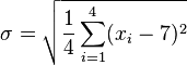
Step 2. Calculate the standard deviation $\sigma\,\!$ :

$\sigma = \sqrt{\frac{1}{N} \sum_{i=1}^N (x_i - \overline{x})^2}$

$\sigma = \sqrt{\frac{1}{4} \sum_{i=1}^4 (x_i - \overline{x})^2}$ Replacing N with 4

$\sigma = \sqrt{\frac{1}{4} \sum_{i=1}^4 (x_i - 7)^2}$ Replacing $\overline{x}$ with 7

$\sigma = \sqrt{\frac{1}{4} \left [ (x_1 - 7)^2 + (x_2 - 7)^2 + (x_3 - 7)^2 + (x_4 - 7)^2 \right ] }$

$\sigma = \sqrt{\frac{1}{4} \left [ (5 - 7)^2 + (6 - 7)^2 + (8 - 7)^2 + (9 - 7)^2 \right ] }$

$\sigma = \sqrt{\frac{1}{4} \left ( (-2)^2 + (-1)^2 + 1^2 + 2^2 \right ) }$

$\sigma = \sqrt{\frac{1}{4} \left ( 4 + 1 + 1 + 4 \right ) }$

$\sigma = \sqrt{\frac{10}{4}}$

$\sigma = \sqrt{\frac{5}{2}} \approx 1.58$

So, the standard deviation is the square root of five halves, or approximately 1.58.

Were this set a sample drawn from a larger population of children, and the question at hand was the standard deviation of the population, convention would replace the denominator N (or 4) in step 2 here with N−1 (or 3).

[edit] Interpretation and application

A large standard deviation indicates that the data points are far from the mean and a small standard deviation indicates that they are clustered closely around the mean.

For example, each of the three data sets {0, 0, 14, 14}, {0, 6, 8, 14} and {6, 6, 8, 8} has a mean of 7. Their standard deviations are 7, 5, and 1, respectively. The third set has a much smaller standard deviation than the other two because its values are all close to 7. In a loose sense, the standard deviation tells us how far from the mean the data points tend to be. It will have the same units as the data points themselves. If, for instance, the data set {0, 6, 8, 14} represents the ages of four siblings, the standard deviation is 5 years.

As another example, the data set {1000, 1006, 1008, 1014} may represent the distances traveled by four athletes in 3 minutes, measured in meters. It has a mean of 1007 meters, and a standard deviation of 5 meters.

Standard deviation may serve as a measure of uncertainty. In physical science for example, the reported standard deviation of a group of repeated measurements should give the precision of those measurements. When deciding whether measurements agree with a theoretical prediction, the standard deviation of those measurements is of crucial importance: if the mean of the measurements is too far away from the prediction (with the distance measured in standard deviations), then we consider the measurements as contradicting the prediction. This makes sense since they fall outside the range of values that could reasonably be expected to occur if the prediction were correct and the standard deviation appropriately quantified. See prediction interval.

[edit] Real-life examples

The practical value of understanding the standard deviation of a set of values is in appreciating how much variation there is away from the "average" (mean).

[edit] Weather

As a simple example, consider average temperatures for cities. While two cities may each have an average temperature of 60 °F, it's helpful to understand that the range for cities near the coast is smaller than for cities inland, which clarifies that, while the average is similar, the chance for variation is greater inland than near the coast.

So, an average of 60 occurs for one city with highs of 80 °F and lows of 40 °F, and also occurs for another city with highs of 65 and lows of 55. The standard deviation allows us to recognize that the average for the city with the wider variation, and thus a higher standard deviation, will not offer as reliable a prediction of temperature as the city with the smaller variation and lower standard deviation.

[edit] Sports

Another way of seeing it is to consider sports teams. In any set of categories, there will be teams that rate highly at some things and poorly at others. Chances are, the teams that lead in the standings will not show such disparity, but will be pretty good in most categories. The lower the standard deviation of their ratings in each category, the more balanced and consistent they might be. So, a team that is consistently bad in most categories will have a low standard deviation indicating they will probably lose more often than win. A team that is consistently good in most categories will also have a low standard deviation and will therefore end up winning more than losing. A team with a high standard deviation might be the type of team that scores a lot (strong offense) but gets scored on a lot too (weak defense); or vice versa, might have a poor offense, but compensate by being difficult to score on - teams with a higher standard deviation will be more unpredictable.

Trying to predict which teams, on any given day, will win, may include looking at the standard deviations of the various team "stats" ratings, in which anomalies can match strengths vs weaknesses to attempt to understand what factors may prevail as stronger indicators of eventual scoring outcomes.

In racing, a driver is timed on successive laps. A driver with a low standard deviation of lap times is more consistent than a driver with a higher standard deviation. This information can be used to help understand where opportunities might be found to reduce lap times.

[edit] Finance

In finance, standard deviation is a representation of the risk associated with a given security (stocks, bonds, property, etc.), or the risk of a portfolio of securities. Risk is an important factor in determining how to efficiently manage a portfolio of investments because it determines the variation in returns on the asset and/or portfolio and gives investors a mathematical basis for investment decisions. The overall concept of risk is that as it increases, the expected return on the asset will increase as a result of the risk premium earned - in other words, investors should expect a higher return on an investment when said investment carries a higher level of risk.

For example, you have a choice between two stocks: Stock A historically returns 5% with a standard deviation of 10%, while Stock B returns 6% and carries a standard deviation of 20%. On the basis of risk and return, an investor may decide that Stock A is the better choice, because the additional percentage point of return (an additional 20% in dollar terms) generated by Stock B is not worth double the degree of risk associated with Stock A. Stock B is likely to fall short of the initial investment more often than Stock A under the same circumstances, and will return only one percentage point more on average. In this example, Stock A has the potential to earn 10% more than the expected return, but is equally likely to earn 10% less than the expected return.

Calculating the average return (or arithmetic mean) of a security over a given number of periods will generate an expected return on the asset. For each period, subtracting the expected return from the actual return results in the variance. Square the variance in each period to find the effect of the result on the overall risk of the asset. The larger the variance in a period, the greater risk the security carries. Taking the average of the squared variances results in the measurement of overall units of risk associated with the asset. Finding the square root of this variance will result in the standard deviation of the investment tool in question. Use this measurement, combined with the average return on the security, as a basis for comparing securities.

[edit] Geometric interpretation

To gain some geometric insights, we will start with a population of three values, x₁, x₂, x₃. This defines a point P = (x₁, x₂, x₃) in R³. Consider the line L = {(r, r, r) : r in R}. This is the "main diagonal" going through the origin. If our three given values were all equal, then the standard deviation would be zero and P would lie on L. So it is not unreasonable to assume that the standard deviation is related to the distance of P to L. And that is indeed the case. Moving orthogonally from P to the line L, one hits the point:

$R = (\overline{x},\overline{x},\overline{x})$

whose coordinates are the mean of the values we started out with. A little algebra shows that the distance between P and R (which is the same as the distance between P and the line L) is given by σ√3. An analogous formula (with 3 replaced by N) is also valid for a population of N values; we then have to work in R^N.

[edit] Rules for normally distributed data

Dark blue is less than one standard deviation from the mean. For the normal distribution, this accounts for 68.27 % of the set; while two standard deviations from the mean (medium and dark blue) account for 95.45 %; and three standard deviations (light, medium, and dark blue) account for 99.73 %.

In practice, one often assumes that the data are from an approximately normally distributed population. This is frequently justified by the classical central limit theorem, which says that sums of many independent, identically-distributed random variables tend towards the normal distribution as a limit. If that assumption is justified, then about 68 % of the values are within 1 standard deviation of the mean, about 95 % of the values are within two standard deviations and about 99.7 % lie within 3 standard deviations. This is known as the 68-95-99.7 rule, or the empirical rule

The confidence intervals are as follows:

σ	68.26894921371%
2σ	95.44997361036%
3σ	99.73002039367%
4σ	99.99366575163%
5σ	99.99994266969%
6σ	99.99999980268%
7σ	99.99999999974%

For normal distributions, the two points of the curve which are one standard deviation from the mean are also the inflection points.

[edit] Chebyshev's inequality

Chebyshev's inequality proves that in any data set, nearly all of the values will be nearer to the mean value, where the meaning of "close to" is specified by the standard deviation. Chebyshev's inequality entails that for (nearly) all random distributions, not just normal ones, we have the following weaker bounds:

At least 50% of the values are within 1.41 standard deviations from the mean.

At least 75% of the values are within 2 standard deviations from the mean.

At least 89% of the values are within 3 standard deviations from the mean.

At least 94% of the values are within 4 standard deviations from the mean.

At least 96% of the values are within 5 standard deviations from the mean.

At least 97% of the values are within 6 standard deviations from the mean.

At least 98% of the values are within 7 standard deviations from the mean.

And in general:

At least (1 − 1/k²) × 100% of the values are within k standard deviations from the mean.

[edit] Relationship between standard deviation and mean

The mean and the standard deviation of a set of data are usually reported together. In a certain sense, the standard deviation is a "natural" measure of statistical dispersion if the center of the data is measured about the mean. This is because the standard deviation from the mean is smaller than from any other point. The precise statement is the following: suppose x₁, ..., x_n are real numbers and define the function:

$\sigma(r) = \sqrt{\frac{1}{N} \sum_{i=1}^N (x_i - r)^2}$

Using calculus, it is possible to show that σ(r) has a unique minimum at the mean:

$r = \overline{x}$

(This can also be done with fairly simple algebra alone, since $σ 2 (r)$ is equated to a quadratic polynomial).

The coefficient of variation of a sample is the ratio of the standard deviation to the mean. It is a dimensionless number that can be used to compare the amount of variance between populations with different means.

[edit] Rapid calculation methods

A slightly faster (significantly for running standard deviation) way to compute the population standard deviation is given by the following formula (though considerations must be made for round-off error, arithmetic overflow, and arithmetic underflow conditions):

$\sigma\ = \sqrt{\left(\frac{1}{N}\sum_{i=1}^N{{x_i}^2}\right) - \overline{x}^2} = \sqrt{\left(\frac{1}{N}\sum_{i=1}^N{{x_i}^2}\right) - \left(\frac{1}{N}\sum_{i=1}^N{{x_i}}\right)^2} = \frac{1}{N}\sqrt{N\left(\sum_{i=1}^N{{x_i}^2}\right) - \left(\sum_{i=1}^N{{x_i}}\right)^2}$