理解距（数学）

 

In mathematics, a moment is, loosely speaking, a quantitative measure of the shape of a set of points. The "second moment", for example, is widely used and measures the "width" (in a particular sense) of a set of points in one dimension or in higher dimensions measures the shape of a cloud of points as it could be fit by an ellipsoid. Other moments describe other aspects of a distribution such as how the distribution is skewed from its mean, or peaked. The mathematical concept is closely related to the concept of moment in physics, although moment in physics is often represented somewhat differently. Any distribution can be characterized by a number of features (such as the mean, the variance, the skewness, etc.), and the moments of a function^[1] describe the nature of its distribution.

The 1st moment is denoted by μ₁. The first moment of the distribution of the random variable X is the expectation operator, i.e., the population mean (if the first moment exists).

In higher orders, the central moments (moments about the mean) are more interesting than the moments about zero. The kth central moment, of a real-valued random variable probability distribution X, with the expected value μ is:

The first central moment is thus 0. The zero-th central moment, μ₀ is one. See also central moment.

Significance of the moments 距的重要性

The n^th moment of a real-valued continuous function f(x) of a real variable about a value c is

It is possible to define moments for random variables in a more general fashion than moments for real values—see moments in metric spaces. The moment of a function, without further explanation, usually refers to the above expression with c = 0.

Usually, except in the special context of the problem of moments, the function f(x) will be a probability density function. The n^th moment about zero of a probability density function f(x) is the expected value of Xⁿ and is called a raw moment or crude moment.^[2] The moments about its mean μ are called central moments; these describe the shape of the function, independently of translation.

If f is a probability density function, then the value of the integral above is called the nth moment of the probability distribution. More generally, if F is a cumulative probability distribution function of any probability distribution, which may not have a density function, then the nth moment of the probability distribution is given by the Riemann–Stieltjes integral

where X is a random variable that has this distribution and E the expectation operator or mean.

When

then the moment is said not to exist. If the nth moment about any point exists, so does (n − 1)th moment, and all lower-order moments, about every point.

Variance方差

Main article: Variance

The second central moment about the mean is the variance, the positive square root of which is the standard deviation σ.

Normalized moments 正规距

The normalized nth central moment or standardized moment is the nth central moment divided by σⁿ; the normalized nth central moment of x = E((x − μ)ⁿ)/σⁿ. These normalized central moments are dimensionless quantities, which represent the distribution independently of any linear change of scale.

Skewness 偏态

Main article: Skewness

The third central moment is a measure of the lopsidedness of the distribution; any symmetric distribution will have a third central moment, if defined, of zero. The normalized third central moment is called the skewness, often γ. A distribution that is skewed to the left (the tail of the distribution is heavier on the left) will have a negative skewness. A distribution that is skewed to the right (the tail of the distribution is heavier on the right), will have a positive skewness.

For distributions that are not too different from the normal distribution, the median will be somewhere near μ − γσ/6; the mode about μ − γσ/2.

Kurtosis 峰态

Main article: Kurtosis

The fourth central moment is a measure of whether the distribution is tall and skinny or short and squat, compared to the normal distribution of the same variance. Since it is the expectation of a fourth power, the fourth central moment, where defined, is always non-negative; and except for a point distribution, it is always strictly positive. The fourth central moment of a normal distribution is 3σ⁴.

The kurtosis κ is defined to be the normalized fourth central moment minus 3. (Equivalently, as in the next section, it is the fourth cumulant divided by the square of the variance.) Some authorities^[3][4] do not subtract three, but it is usually more convenient to have the normal distribution at the origin of coordinates. If a distribution has a peak at the mean and long tails, the fourth moment will be high and the kurtosis positive (leptokurtic); and conversely; thus, bounded distributions tend to have low kurtosis (platykurtic).

The kurtosis can be positive without limit, but κ must be greater than or equal to γ² − 2; equality only holds for binary distributions. For unbounded skew distributions not too far from normal, κ tends to be somewhere in the area of γ² and 2γ².

The inequality can be proven by considering

where T = (X − μ)/σ. This is the expectation of a square, so it is non-negative whatever a is; on the other hand, it's also a quadratic equation in a. Its discriminant must be non-positive, which gives the required relationship.

Mixed moments 混合距

Mixed moments are moments involving multiple variables.

Some examples are covariance, coskewness and cokurtosis. While there is a unique covariance, there are multiple co-skewnesses and co-kurtoses.

Higher moments 高阶距

High-order moments are moments beyond 4th-order moments. The higher the moment, the harder it is to estimate, in the sense that larger samples are required in order to obtain estimates of similar quality.^{[citation needed]}

Cumulants 累积距

Main article: cumulant

The first moment and the second and third unnormalized central moments are additive in the sense that if X and Y are independent random variables then

and

and

(These can also hold for variables that satisfy weaker conditions than independence. The first always holds; if the second holds, the variables are called uncorrelated).

In fact, these are the first three cumulants and all cumulants share this additivity property.

Sample moments 样本距

The moments of a population can be estimated using the sample k-th moment

applied to a sample X₁,X₂,..., X_n drawn from the population.

It can be shown that the expected value of the sample moment is equal to the k-th moment of the population, if that moment exists, for any sample size n. It is thus an unbiased estimator.

Problem of moments 距的问题

The problem of moments seeks characterizations of sequences { μ′_n : n = 1, 2, 3, ... } that are sequences of moments of some function f.

Partial moments 部分距/一边距

Partial moments are sometimes referred to as "one-sided moments." The nth order lower and upper partial moments with respect to a reference point r may be expressed as

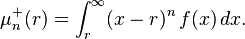
Partial moments are normalized by being raised to the power 1/n. The upside potential ratio may be expressed as a ratio of a first-order upper partial moment to a normalized second-order lower partial moment.

Moments in metric spaces 矩阵空间中的距

Let (M, d) be a metric space, and let B(M) be the Borel σ-algebra on M, the σ-algebra generated by the d-open subsets of M. (For technical reasons, it is also convenient to assume that M is a separable space with respect to the metric d.) Let 1 ≤ p ≤ +∞.

The p^th moment of a measure μ on the measurable space (M, B(M)) about a given point x₀ in M is defined to be

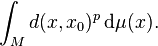
μ is said to have finite p^th moment if the p^th moment of μ about x₀ is finite for some x₀ ∈ M.

This terminology for measures carries over to random variables in the usual way: if (Ω, Σ, P) is a probability space and X : Ω → M is a random variable, then the p^th moment of X about x₀ ∈ M is defined to be

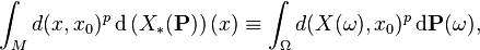
and X has finite p^th moment if the p^th moment of X about x₀ is finite for some x₀ ∈ M.

 

 

 

http://en.wikipedia.org/wiki/Moment_(mathematics)