

卷积神经网络 Convolutional Neural Networks (LeNet)
CNN(卷积神经网络)是传统神经网络的变种,CNN在传统神经网络的基础上,引入了卷积和pooling。与传统的神经网络相比,CNN更适合用于图像中,卷积和图像的局部特征相对应,pooling使得通过卷积获得的feature具有空间不变性
接触的最多的卷积应该是高斯核,用于对图像进行平滑,或者是实现在不同尺度下的运算等。这里的卷积和高斯核是同一个类型,就是定义了一个卷积的尺度,然后卷积的具体参数就是神经网络中的参数,通过计算神经网络的参数,相当于学到了多个卷积的参数,而每个卷积可以看成是对图像进行特征提取(一个特征核),CNN网络就可以看成是前面的几层都是在提取图像的特征,最后一层$softmax$用于对提取的特征进行分类。所有CNN的特征是自学习(相对于SIFT,SURF)
conv2d是theano中的用于计算卷积的方法(theano.tensor.conv2($input$, $W$)),其中$W$表示卷积核。$W$是必须是一个4D的tensor(T.tensor4),$input$也必须是一个4D的tensor。
下面说下$input$和$W$中每个维度分别表示的意义。
$input \in (batches, feature, I_h, I_w)$分别表示batch size,number of feature map, image height ,image width
$W \in (filters, feature, f_h, f_w)$ 分别表示number of filters, number of feature map, filter height, filter width
其中$W_{shape[1]}$必须等于$input_{shape[1]}$。$W_{shape[1]} = 1$表示这个filter是在2D空间中的filter,$W_{shape[1]} > 1$表示这个filter是3D中间中的filter,如果$W_{shape[1]} = 3$这是这个filter是图像3通道上的filter,3个通道上进行卷积。
\begin{equation} input \in (batches, feature, I_h, I_w) \\ W \in (filters, feature, f_h, f_w) \end{equation}
\begin{equation} output = input \otimes W \\ output \in (batches, filters , I_h - f_h + 1, I_w - f_w + 1) \end{equation}
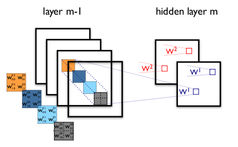
Pooling是在二维空间中操作的,如上图所示,将特征按照空间位置分成大的block,然后再每个block中计算特征。$max pooling$就是在这个block中计算所有位置的最大值作为特征,$average pooling$为计算区域内的特征均值
为什么需要pooling,图像分类中的BOW也适用了Pooling。我认为,在CNN中适用pooling的好处主要有两点:
1.如果不使用pooling,那么通过卷积计算得到的隐层节点的个数是卷积类型的倍数。举个例子:如上面的$input$,和$W$,$input$中每个patch的输入节点个数为$feature \times I_h \times I_w$,通过$W$的卷积运算后,$output$的节点数目为$filters \times (I_h - f_h + 1) \times (I_w - f_w + 1)$,如果引入pooling策略,$output$的节点数目就变为$filters \times \frac{I_h - f_h + 1}{p_h} \times \frac{I_w - f_w + 1}{p_w}$其中$p_h, p_w$表示pooling中每个区域的大小。从而减少了隐含层节点的个数,降低了计算复杂度。
2.引入pooling的另外一个好处就是使得CNN的模型具有局部区域内的平移或者旋转的一些不变性。很多精心设计的特征,如SIFT,SURF,HOG等等都具有这些不变性。不变性使得CNN在图像分类的问题中能够大方光彩,取得较好的performance。
在theano中,用于计算pooling的函数为$\text{theano.tensor.signal.downsample.max_pool_2d}$。对一个$N(N \geq 2)$维的输入矩阵,通过定义$p_h, p_w$然后对输入数据进行pooling
在Deep Learning tutorial的Convolutional Neural Network(LeNet)中,改例子用于MNIST数据集的字符识别(10个类别,识别阿拉伯数字),每个字符为$28\times28$的像素的输入,50000个样本用于训练,10000个样本用于交叉验证,另外10000个用于测试。可以在这里下载MNIST,另外,模型采用基于mini-batch的SGD进行优化。
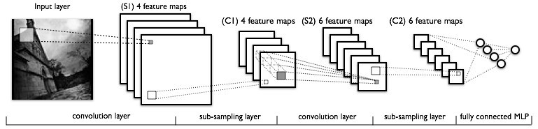
这个用于识别手写数字的CDNN模型的结构是这样过如最前面那个图所示。
输入层:每个mini-batch的原始图像$image shape = (batch size, 1, 28, 28)$
layer0_input = x.reshape((batch_size, 1, 28, 28))
卷积层1:对于输入的每个mini-batch的数据,output为卷积+pooling处理后的结果,第一层卷积类型为$nkerns[0]=20$个,卷积核的尺度为$f_h = 5, f_w = 5$
pooling的尺度为$(2,2)$
通过卷积,$filtershape=(nkerns[0],1,5,5)$,图像的尺度变化$(I_h -f_h + 1, I_w - f_w +1) \to (28, 28) ---> (24,24)$
通过pooling后$(24, 24) ---> (24/2,24/2)$
feature map的维度变为卷积类型数,所有$outputshape=(batch size, nkerns[0], 12, 12)$
layer0 = LeNetConvPoolLayer(rng, input=layer0_input,
                                image_shape=(batch_size,1,28,28),
                                filter_shape=(nkerns[0], 1, 5, 5), poolsize=(2,2))
卷积层2:输入为卷积层1的输出,所以$inputsize=(batch size, nkerns[0], 12, 12)$
通过卷积,$filtershape=(nkerns[1],nkerns[0],5,5)$,图像的尺度变化$(I_h -f_h + 1, I_w - f_w +1) \to (12, 12) ---> (8, 8)$
通过pooling后$(8, 8) ---> (8/2, 8/2)$
feature map的维度变为卷积类型数,所有$outputshape=(batch size, nkerns[1], 4, 4)$
layer1 = LeNetConvPoolLayer(rng, input=layer0.output,
                                image_shape=(batch_size, nkerns[0], 12, 12),
                                filter_shape=(nkerns[1], nkerns[0], 5,5), poolsize=(2,2))
全连接层:输入为卷积层2的输出,并将输入转化为$1D$的向量,所以$inputsize=nkerns[1]*4*4$
该层为普通的全连接层,和普通的神经网络一样,输入层的每个节点都与输出层的每个节点相连接
输出层的output节点个数在这里设置为$500$
Layer2_input = layer1.output.flatten(2)
# construct a fully-connected sigmoidal layer
layer2 = HiddenLayer(rng, input=Layer2_input, n_in=nkerns[1]*4*4, n_out=500, activation=T.tanh)
SoftMax层:最后一层是用于分类的softmax层,输入为上一层的输出,$input=500$
输出层的Classification的类别数,在这里为10。
# classify the values of the fully-connected sigmoidal layer
    layer3 = LogisticRegression(input=layer2.output, n_in=500, n_out=10)
(1) import部分
import sys
import time
import theano
import theano.tensor as T
import numpy as np
from theano.tensor.nnet import conv
from theano.tensor.signal import downsample
from LogistRegression import LogisticRegression, load_data
from mlp import HiddenLayer
(2) LeNetConvPoolLayer的定义部分
$input:$表示输入数据
$rng:$卷积核的随机函数种子
$filtershape:$卷积核的参数维度
$imageshape:$输入数据的维度
值得一提的是初始化参数的设置方法,一种方式如下:
$fanin:$每个输出节点需要多少个input进行输入,这种方式没有考虑maxpooling
        fan_in = np.prod(filter_shape[1:])
        W_values = np.asarray(rng.uniform(
            low=-np.sqrt(3./fan_in),
            high=np.sqrt(3./fan_in),
            size=filter_shape), dtype=theano.config.floatX)
        self.W = theano.shared(value=W_values, name='W')
另外一种方式为
        fan_in = np.prod(filter_shape[1:])
        # each unit in the lower layer receives a gradient from:
        # "num output feature maps * filter height * filter width" /
        #   pooling size
        fan_out = (filter_shape[0] * np.prod(filter_shape[2:])/np.prod(poolsize))
        # initialize weights with random weights
        W_bound = np.sqrt(6. / (fan_in + fan_out))
        W_values = np.asarray(rng.uniform(
            low=-W_bound,
            high=W_bound,
            size=filter_shape), dtype=theano.config.floatX)
$fanin:$和第一种方式一样,只不过这里多了$fanout$
如果不考虑pooling,那么$fanout=filter_shape[0]*np.prod(filter_shape[2:])$
考虑了pooling之后,$fanout=filter_shape[0]*np.prod(filter_shape[2:])/np.prod(poolsize)$
class LeNetConvPoolLayer(object):

	def __init__(self, rng, input, filter_shape, image_shape, poolsize=(2,2)):
		"""
		Alloc a LeNetConvPoolLayer with shared variable internal parameters

		:type rng: numpy.random.RandomState
		:param rng: a random number generator used to initilize weights

		:type input: theano.tensor.dtensor4
		:param input: symbolic image tensor, of shape image_shape

		:type filter_shape: tuple or list of length 4
		:param filter_shape: (number of filters, num input feature maps, filter height, filter width)

		:type image_shape: tuple or list of length 4
		:param image_shape: (batch size, num input feature maps, image height, image width)

		:type poolsize: tuple or list of length 2
		:param poolsize: the downsampling (pooling) factor (#rows, #cols)

		"""

		# why ? pleas look for http://www.cnblogs.com/cvision/p/3276577.html
		assert image_shape[1] == filter_shape[1]
		self.input = input

		# initilize weights values: the fan-in of each hidden neuron is
		# restrited by the size of the receptive fields
		"""
		fan_in = np.prod(filter_shape[1:])
		W_values = np.asarray(rng.uniform(
			low=-np.sqrt(3./fan_in),
			high=np.sqrt(3./fan_in),
			size=filter_shape), dtype=theano.config.floatX)
		self.W = theano.shared(value=W_values, name='W')
		"""

		fan_in = np.prod(filter_shape[1:])
        # each unit in the lower layer receives a gradient from:
        # "num output feature maps * filter height * filter width" /
        #   pooling size
		fan_out = (filter_shape[0] * np.prod(filter_shape[2:])/np.prod(poolsize))
        # initialize weights with random weights
		W_bound = np.sqrt(6. / (fan_in + fan_out))
		W_values = np.asarray(rng.uniform(
			low=-W_bound,
			high=W_bound,
			size=filter_shape), dtype=theano.config.floatX)
		self.W = theano.shared(value=W_values, name='W')
		#print self.W.get_value()
		# the bias is a 1D theano -- one bias per output feature map
		b_values = np.zeros((filter_shape[0],),dtype=theano.config.floatX);
		self.b = theano.shared(value=b_values, name='b')

		# convolve input feature maps with filters
		conv_out = conv.conv2d(input, self.W, filter_shape=filter_shape, image_shape=image_shape)

		# downsample each feature map individually, using maxpooling
		pooled_out = downsample.max_pool_2d(conv_out, poolsize, ignore_border=True)

		# add the bias term. Since the bias term is a vector(1D array), we first
		# reshape it to a tensor of shape(1, n_filters, 1, 1). Each bias will
		# thus be broadcasted across mini-batches and feature map with & height
		self.output = T.tanh(pooled_out + self.b.dimshuffle('x', 0, 'x', 'x'))

		self.params = [self.W, self.b]
(3) LeNet网络结构定义
首先将数据处理成patch的格式,在这里是通过patch_index来实现的
n_train_batches = train_set_x.get_value(borrow=True).shape[0] / batch_size
    n_valid_batches = valid_set_x.get_value(borrow=True).shape[0] / batch_size
    n_test_batches = test_set_x.get_value(borrow=True).shape[0] / batch_size
具体代码如下
def evaluate_lenet5(learning_rate=0.1, n_epochs=200,dataset = './data/mnist.pkl.gz',
					nkerns=[20, 50], batch_size=500):
	""" Demostartes lenet on MNIST dataset

	:type learning_rate: float
	:param learning_rate: learning rate used(factor for the stochastic gradient)

	:type n_epochs: int
	:param n_epochs: maximal number of epochs to run the optimizer

	:type dataset: string
	:param dataset: path to the dataset used for training / testing

	:type nkerns: list of ints
	:param nkerns: number of kernels on each LeNetConvPoolLayer

	:type batch_size : int
	:param batch_size : size of data in  each batch
	"""

	#used for LeNetConvPoolLayer to random the filter weights
	rng = np.random.RandomState(23455)

	datasets = load_data(dataset)

	print >> sys.stdout, '...load data is ok'

	# get train_set vaild_set and test set
	train_set_x, train_set_y = datasets[0]
	valid_set_x, valid_set_y = datasets[1]
	test_set_x, test_set_y = datasets[2]

	# calculate there are how many batches
	n_train_batches = train_set_x.get_value(borrow=True).shape[0] / batch_size
	n_valid_batches = valid_set_x.get_value(borrow=True).shape[0] / batch_size
	n_test_batches = test_set_x.get_value(borrow=True).shape[0] / batch_size


	#print "n_train_batches = %d n_valid_batches = %d n_test_batches = %d" %(train_set_x.get_value(borrow=True).shape[0],
	#	valid_set_x.get_value(borrow=True).shape[0],test_set_x.get_value(borrow=True).shape[0])
	######################
	# BUILD ACTUAL MODEL #
	######################

	print '...building the model'

	index = T.lscalar() # index to [mini]batches
	x = T.matrix('x')   # images
	y = T.ivector('y')  # the labels

	ishape = (28, 28)   # the size of MNIST images

	# Reshape matrix of images of shape(batches, 28 * 28)
	# to a 4D tensor, compatible with our LeNetConvPoolLayer

	layer0_input = x.reshape((batch_size, 1, 28, 28))

	# Construct the first convolutional pooling layer:
	# filtering reduce the image size to (I_h - f_h + 1, I_w - f_w + 1)
	# this problem is (28, 28)---->(28-5+1, 28-5+1)=(24,24)
	# maxpooling reduces this futher to (24/2, 24/2)= (12, 12)
	# so the 4D output tensor is thus of shape (batch_size, nkerns[0], 12, 12)

	layer0 = LeNetConvPoolLayer(rng, input=layer0_input,
								image_shape=(batch_size,1,28,28),
								filter_shape=(nkerns[0], 1, 5, 5), poolsize=(2,2))

	# Construct the first convolutional pooling layer:
	# filtering reduces the image size to (12-5+1, 12-5+1) = (8, 8)
	# max pooling reduces this futert to (8/2, 8/2)=(4,4)
	# 4D output tensor is thus of shape (batch_size, nkerns[1], 4, 4)
	layer1 = LeNetConvPoolLayer(rng, input=layer0.output,
								image_shape=(batch_size, nkerns[0], 12, 12),
								filter_shape=(nkerns[1], nkerns[0], 5,5), poolsize=(2,2))

	# the TanhLayer being full-connected,it operates on 2D matrices of
	# the shape (batches, num_pixels) (i.e matrix of rasterized images)
	# This will generate a matrix of (batches, nkerns[1]*4*4)

	Layer2_input = layer1.output.flatten(2)

	# construct a fully-connected sigmoidal layer
	layer2 = HiddenLayer(rng, input=Layer2_input, n_in=nkerns[1]*4*4, n_out=500, activation=T.tanh)

	# classify the values of the fully-connected sigmoidal layer
	layer3 = LogisticRegression(input=layer2.output, n_in=500, n_out=10)
(4) Mini-batch SGD优化
定义用于优化的损失函数$NLL$
\begin{equation}
\frac{1}{|\mathcal{D}|}\mathcal{L}(\theta=\{W,b\},\mathcal{D})=\frac{1}
{|\mathcal{D}|}\sum_{i=0}^{|\mathcal{D}|} \log{P(Y=y^{(i)}|x^{(i)}, W, B)} \\
\ell (\theta=\{W,b\},\mathcal{D}) = - \frac{1}{|\mathcal{D}|}\mathcal{L}
(\theta=\{W,b\},\mathcal{D})
\end{equation}
# the cost we minimize during training is the NLL of the model
    cost = layer3.negative_log_likelihood(y)
定义用于测试当前模型在Validation和Testing集合中的性能的函数
# create a function to compute the msitaken that are made by the model
    test_model = theano.function([index], layer3.errors(y),
        givens={
            x:test_set_x[index*batch_size:(index+1)*batch_size],
            y:test_set_y[index*batch_size:(index+1)*batch_size]})

    validate_model = theano.function([index], layer3.errors(y),
        givens={
            x:valid_set_x[index*batch_size:(index+1)*batch_size],
            y:valid_set_y[index*batch_size:(index+1)*batch_size]})
定义模型的所有参数以及参数的梯度
# create a list of all model parameters to be fit by gradient descent
    params = layer3.params + layer2.params + layer1.params + layer0.params

    # create a list of gradients for all model parameters
    grads = T.grad(cost, params)
定义SGD的优化策略,梯度更新
updates = []
    for param_i, grad_i in zip(params, grads):
        updates.append((param_i, param_i - learning_rate * grad_i))

    train_model = theano.function(inputs=[index],
                                  outputs=cost,
                                  updates=updates,
                                  givens={
        x:train_set_x[index*batch_size:(index + 1)*batch_size],
        y:train_set_y[index*batch_size:(index + 1)*batch_size]})
总体代码如下
def evaluate_lenet5(learning_rate=0.1, n_epochs=200,dataset = './data/mnist.pkl.gz',
					nkerns=[20, 50], batch_size=500):
	""" Demostartes lenet on MNIST dataset

	:type learning_rate: float
	:param learning_rate: learning rate used(factor for the stochastic gradient)

	:type n_epochs: int
	:param n_epochs: maximal number of epochs to run the optimizer

	:type dataset: string
	:param dataset: path to the dataset used for training / testing

	:type nkerns: list of ints
	:param nkerns: number of kernels on each LeNetConvPoolLayer

	:type batch_size : int
	:param batch_size : size of data in  each batch
	"""

	#used for LeNetConvPoolLayer to random the filter weights
	rng = np.random.RandomState(23455)

	datasets = load_data(dataset)

	print >> sys.stdout, '...load data is ok'

	# get train_set vaild_set and test set
	train_set_x, train_set_y = datasets[0]
	valid_set_x, valid_set_y = datasets[1]
	test_set_x, test_set_y = datasets[2]

	# calculate there are how many batches
	n_train_batches = train_set_x.get_value(borrow=True).shape[0] / batch_size
	n_valid_batches = valid_set_x.get_value(borrow=True).shape[0] / batch_size
	n_test_batches = test_set_x.get_value(borrow=True).shape[0] / batch_size


	#print "n_train_batches = %d n_valid_batches = %d n_test_batches = %d" %(train_set_x.get_value(borrow=True).shape[0],
	#	valid_set_x.get_value(borrow=True).shape[0],test_set_x.get_value(borrow=True).shape[0])
	######################
	# BUILD ACTUAL MODEL #
	######################

	print '...building the model'

	index = T.lscalar() # index to [mini]batches
	x = T.matrix('x')   # images
	y = T.ivector('y')  # the labels

	ishape = (28, 28)   # the size of MNIST images

	# Reshape matrix of images of shape(batches, 28 * 28)
	# to a 4D tensor, compatible with our LeNetConvPoolLayer

	layer0_input = x.reshape((batch_size, 1, 28, 28))

	# Construct the first convolutional pooling layer:
	# filtering reduce the image size to (I_h - f_h + 1, I_w - f_w + 1)
	# this problem is (28, 28)---->(28-5+1, 28-5+1)=(24,24)
	# maxpooling reduces this futher to (24/2, 24/2)= (12, 12)
	# so the 4D output tensor is thus of shape (batch_size, nkerns[0], 12, 12)

	layer0 = LeNetConvPoolLayer(rng, input=layer0_input,
								image_shape=(batch_size,1,28,28),
								filter_shape=(nkerns[0], 1, 5, 5), poolsize=(2,2))

	# Construct the first convolutional pooling layer:
	# filtering reduces the image size to (12-5+1, 12-5+1) = (8, 8)
	# max pooling reduces this futert to (8/2, 8/2)=(4,4)
	# 4D output tensor is thus of shape (batch_size, nkerns[1], 4, 4)
	layer1 = LeNetConvPoolLayer(rng, input=layer0.output,
								image_shape=(batch_size, nkerns[0], 12, 12),
								filter_shape=(nkerns[1], nkerns[0], 5,5), poolsize=(2,2))

	# the TanhLayer being full-connected,it operates on 2D matrices of
	# the shape (batches, num_pixels) (i.e matrix of rasterized images)
	# This will generate a matrix of (batches, nkerns[1]*4*4)

	Layer2_input = layer1.output.flatten(2)

	# construct a fully-connected sigmoidal layer
	layer2 = HiddenLayer(rng, input=Layer2_input, n_in=nkerns[1]*4*4, n_out=500, activation=T.tanh)

	# classify the values of the fully-connected sigmoidal layer
	layer3 = LogisticRegression(input=layer2.output, n_in=500, n_out=10)

	# the cost we minimize during training is the NLL of the model
	cost = layer3.negative_log_likelihood(y)

	# create a function to compute the msitaken that are made by the model
	test_model = theano.function([index], layer3.errors(y),
		givens={
			x:test_set_x[index*batch_size:(index+1)*batch_size],
			y:test_set_y[index*batch_size:(index+1)*batch_size]})

	validate_model = theano.function([index], layer3.errors(y),
		givens={
			x:valid_set_x[index*batch_size:(index+1)*batch_size],
			y:valid_set_y[index*batch_size:(index+1)*batch_size]})

	# create a list of all model parameters to be fit by gradient descent
	params = layer3.params + layer2.params + layer1.params + layer0.params

	# create a list of gradients for all model parameters
	grads = T.grad(cost, params)


	# train_model is a function that updates the model parameters by
	# SGD Since this model has many parameters, it would be tedious
	# manually create an update rule for each model paramter. We thus
	# crate updates list by automatically looping over all
	# (params[i].grad[i]) pairs

	updates = []
	for param_i, grad_i in zip(params, grads):
		updates.append((param_i, param_i - learning_rate * grad_i))

	train_model = theano.function(inputs=[index],
								  outputs=cost,
								  updates=updates,
								  givens={
		x:train_set_x[index*batch_size:(index + 1)*batch_size],
		y:train_set_y[index*batch_size:(index + 1)*batch_size]})


###############
	# TRAIN MODEL #
	###############

	print '... training'

	# early-stoping  parameters
	patience = 10000 # look as this many examples regardless
	patience_increase = 2 # wait this much longer when a new best is found
	improvement_threshold = 0.995  # a relative improvement of this much is considered significant
	validation_frequency = min(n_train_batches, patience/2)

	best_params =  None
	best_validation_loss = np.inf
	best_iter = 0
	test_score = 0
	start_time = time.clock()

	epoch = 0
	done_looping = False


	while epoch < n_epochs and (not done_looping):
		epoch = epoch + 1
		for minibatch_index in xrange(n_train_batches):

			minibatch_avg_cost = train_model(minibatch_index)

			iter =  (epoch - 1)  * n_train_batches + minibatch_index

			if ( iter + 1 ) % validation_frequency == 0:
				valication_losses = [validate_model(i)
									for i in xrange(n_valid_batches)]
				this_validation_loss = np.mean(valication_losses)

				print ('epoch %i, minibacth %i/%i, validation error %f %%' % \
				(epoch, minibatch_index + 1 , n_train_batches, this_validation_loss * 100.))

				if this_validation_loss < best_validation_loss:
					if this_validation_loss < best_validation_loss * improvement_threshold:
						patience = max(patience, iter * patience_increase)

					best_validation_loss = this_validation_loss

					# test it on the test set
					best_iter = iter
					test_losses = [test_model(i) for i in xrange(n_test_batches)]
					test_score = np.mean(test_losses)

					print '     patience %d epoch %i, minibatch %i/%i , test error of best model  %f %%' %( patience, epoch,
					minibatch_index + 1, n_train_batches, test_score * 100.)

			if patience <= iter:
				done_looping = True
				break
	end_time = time.clock()
	print 'Optimization complete with best validation score of %f %% with the test performance %f %%' \
	%(best_validation_loss * 100. , test_score * 100.)

	print 'The code run for %d epochs with %f epchos /sec' %(epoch, 1. * epoch / (end_time - start_time))
	print >> sys.stderr, ('The code for file ' +
                          os.path.split(__file__)[1] +
                          ' ran for %.1fs' % ((end_time - start_time)))
Code百度网盘地址[code]

 浙公网安备 33010602011771号