《Text Mining and Analysis》Fourth Week Study Notes

《Text Mining and Analysis》Fourth Week Study Notes

Course Overview:

Goals and Objectives

After you actively engage in the learning experiences in this module, you should be able to:

• Explain the concept of text clustering and why it is useful.
• Explain how we can design a probabilistic generative model for performing text clustering, and explain the similarity and difference between such a model and a topic model such as PLSA.
• Explain how Hierarchical Agglomerative Clustering and k-Means clustering work.
• Explain how to evaluate text clustering.
• Explain the concept of text categorization and why it is useful.
• Explain how Naïve Bayes classifier works.

Guiding Questions

Develop your answers to the following guiding questions while watching the video lectures throughout the week.

• What is clustering? What are some applications of clustering in text mining and analysis?
• How can we use a mixture model to do document clustering? How many parameters are there in such a model?
• How is the mixture model for document clustering related to a topic model such as PLSA? In what way are they similar? Where are they different?
• How do we determine the cluster for each document after estimating all the parameters of a mixture model?
• How does hierarchical agglomerative clustering work? How do single-link, complete-link, and average-link work for computing group similarity? Which of these three ways of computing group similarity is least sensitive to outliers in the data?
• How do we evaluate clustering results?
• What is text categorization? What are some applications of text categorization?
• What does the training data for categorization look like?
• How does the Naïve Bayes classifier work?
• Why do we often use logarithm in the scoring function for Naïve Bayes?

Key Phrases and Concepts

Keep your eyes open for the following key terms or phrases as you complete the readings and interact with the lectures. These topics will help you better understand the content in this module.

• Clustering, document clustering, and term clustering
• Clustering bias
• Perspective of similarity
• Mixture model, likelihood, and maximum likelihood estimation
• EM algorithm, E-step, M-step, underflow, normalization (to avoid underflow)
• Hierarchical Agglomerative Clustering, and k-Means
• Direction evaluation (of clustering), indirect evaluation (of clustering)
• Text categorization, topic categorization, sentiment categorization, email routing
• Spam filtering
• Naïve Bayes classifier
• Smoothing

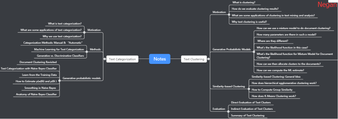
• Text Clustering
  • Motivation
    • What is clustering?　
    • How do we evaluate clustering results?
    • What are some applications of clustering in text mining and analysis?
    • Why text clustering is useful?
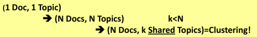
  • Generative Probabilistic Models
    • How can we use a mixture model to do document clustering? 
    • How many parameters are there in such a model?　
    • Where are they different?　
    • What's the likelihood function in this case?
    • What's the likelihood function for Mixture Model for Document Clustering?
    • How can we then allocate clusters to the documents?
    • How can we compute the ML estimate?
  • Similarity-based Clustering 
    • Similarity-based Clustering: General Idea
    • How does hierarchical agglomerative clustering work?
    • How to Compute Group Similarity
    • How does K-Means Clustering work？
  • Evaluation
    • Direct Evaluation of Text Clusters
    • Indirect Evaluation of Text Clusters
    • Summary of Text Clustering
• Text Categorization
  • Motivation
    • What is text categorization?
    • What are some applications of text categorization?
    • Why we use text categorization?
  • Methods
    • Categorization Methods: Manual & “Automatic”
    • Machine Learning for Text Categorization
    • Generative vs. Discriminative Classifiers
  • Generative probabilistic models
    • Document Clustering Revisited
    • Text Categorization with Naïve Bayes Classifier
    • Learn from the Training Data
    • How to Estimate p(w|θi) and p(θi )
    • Smoothing in Naïve Bayes 
    • Anatomy of Naïve Bayes Classifier

1.Text Clustering: Motivation

1.1 What is clustering?　

　　Well, clustering actually is a very general technique for data mining as you might have learned in some other courses. The idea is to discover natural structures in the data.In another words, we want to group similar objects together. In our case, these objects are of course, text objects. You can just see this picture:

　　

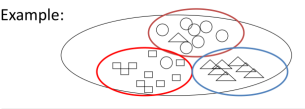
　　And they may not be so much this agreement about these three clusters but it really depends on the perspective to look at the objects. And the problem lies in how to define similarity.So as we can see, it really depends on our perspective, to look at the objects. And so it ought to make the clustering problem well defined. A user must define the perspective for assessing similarity. And we call this perspective the clustering bias. 

1.2 How do we evaluate clustering results?　　

　　So as you can see clearly here, depending on the perspective, we'll get different clustering result. So that also clearly tells us that in order to evaluate the clustering without, we must use perspective. Without perspective, it's very hard to define what is the best clustering result. 

1.3  What are some applications of clustering in text mining and analysis?

　　In the lecture,some applications are listed as follow:　

• Clustering of documents in the whole collection
• Term clustering to define “concept”/“theme”/“topic”
• Clustering of passages/sentences or any selected text segments from larger text objects (e.g., all text segments about a topic discovered using a topic model)
• Clustering of websites (text object has multiple documents)
• Text clusters can be further clustered to generate a hierarchy

1.4 Why text clustering is useful?

　　(1) In general, very useful for text mining and exploratory text analysis:

• Get a sense about the overall content of a collection (e.g., what are some of the “typical”/representative documents in a collection?)
• Link (similar) text objects (e.g., removing duplicated content)
• Create a structure on the text data (e.g., for browsing)
• As a way to induce additional features (i.e., clusters) for classification of text objects

　　(2)Examples of applications

• Clustering of search results
• Understanding major complaints in emails from customers

2.Text Clustering: Generative Probabilistic Models

2.1 How can we use a mixture model to do document clustering? 

　　In the mixture model,the words in the document that could have been generated in general from multiple distributions.

　　Now this is not what we want, as we said, for text clustering, for document clustering, where we hoped this document will be generated from precisely one topic.That's why mixture model cannot be used for clustering because it did not ensure that only one distribution has been used to generate all the words in one document.

　　So if you realize this problem, then we can naturally design alternative mixture model for doing clustering. So this is what you're seeing here. And we again have to make a decision regarding which distribution to use to generate this document because the document could potentially be generated from any of the k word distributions that we have. But this time, once we have made a decision to choose one of the topics, we're going to stay with this regime to generate all the words in the document.

 

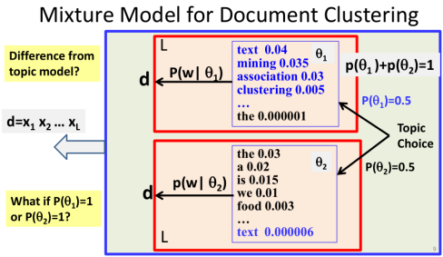
　　And that means, once we have made a choice of the distribution in generating the first word, we're going to go stay with this distribution in generating all of the other words in the document.

2.2 How many parameters are there in such a model?　

　　We no longer have the detailed coverage distributions pi i j. But instead, we're going to have a cluster assignment decisions, Ci. And Ci is a decision for the document i. And C sub i is going to take a value from 1 through k to indicate one of the k clusters.

 

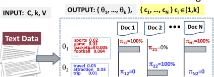
　　And basically tells us that d i is in which cluster. As illustrated here, we no longer have multiple topics covered in each document. It is precisely one topic. We assume a collection of N documents with a fixed number of topics k where the vocabulary size is M. Then there will be N+KM parameters.

 

2.3  Where are they different?　

　　The decision of using a particular distribution is made just once for this document, in the case of document clustering. But in the case of topic model, we have to make as many decisions as the number of words in the document. Because for each word, we can make a potentially different decision. And that's the key difference between the two models.

　　In general,there are mainly two differences, one is the choice of using that particular distribution is made just once for document clustering. Whereas in the topic model, it's made it multiple times for different words. The second is that word distribution, here, is going to be used to regenerate all the words for a document. But, in the case of one distribution doesn't have to generate all the words in 

2.4 What's the likelihood function in this case?　　

　　Let's also think about a special case, when one of the probability of choosing a particular distribution is equal to 1. Now that just means we have no uncertainty now. We just stick with one particular distribution. Now in that case, clearly, we will see this is no longer mixture model, because there's no uncertainty here and we can just use precisely one of the distributions for generating a document. And we're going back to the case of estimating one order distribution based on one document.

　　So as in all cases of using a generative model to solve a problem, we first look at data and then think about how to design the model. But once we design the model, the next step is to write down the likelihood function. And after that we're going to look at the how to estimate the parameters. 

　　The likelihood function:

　　

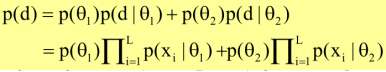
　　In topic model, we see that the sum is actually inside the product.:

 2.5 What's the likelihood function for Mixture Model for Document Clustering?

　　It can be showed as follow:

•  Data: a collection of documents C={d₁ , …, d_N }
•  Model: mixture of k unigram LMs:Λ=({θ_i }; {p(θ_i )}), i[1,k]

　　　　To generate a document, first choose a θ_i according to p(θ_i ), and then generate all words in the document using p(w|θ_i )

• Likelihood:

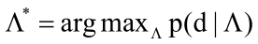
• Maximum Likelihood estimate:

2.6 How can we then allocate clusters to the documents?

　　Once we can estimate the parameters of the model, then we can easily solve the problem of document clustering. It can be showed as follow:

　（1） Parameters of the mixture model: Λ=({θ_i }; {p(θ_i )}), i[1,k]

• Each θ_i represents the content of cluster i : p(w| θ_i)
•  p(θ_i) indicates the size of cluster i
• Note that unlike in PLSA, p(θ_i) doesn’t depend on d!

　（2）Which cluster should document d belong to? c_d =?

• Likelihood only: Assign d to the cluster corresponding to the topic θ_i that most likely has been used to generate d

 

• Likelihood + prior p(θ_i) (Bayesian): favor large clusters

 2.7 How can we compute the ML estimate?

　　We  can compute the ML estimate by EM algorithm.Here is the details:

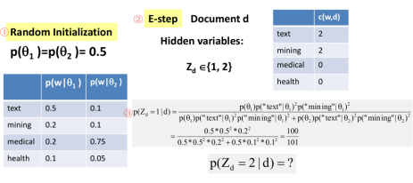
•  Initialization: Randomly set  Λ=({θ_i }; {p(θ_i )}), i[1,k]
•  Repeat until likelihood p(C|Λ ) converges

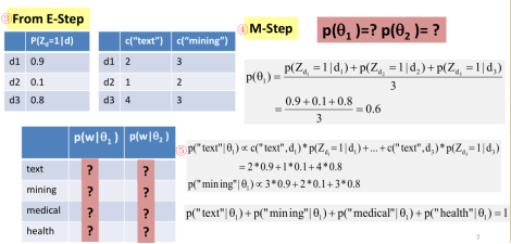
　　　　E-Step: Infer which distribution has been used to generate document d: hidden variable Z_d [1,k]

　　　　 M-Step:  Re-estimation of all parameters

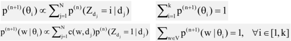
　　Here is a simple example of two clusters.:

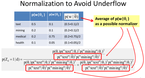
　　Now it's important that you note that in such a computation there is a potential problem of underflow. And that is because if you look at the original numerator and the denominator, it involves the competition of a product of many small probabilities. Imagine if a document has many words and it's going to be a very small value here that can cause the problem of underflow. So to solve the problem, we can use a normalize. So here you see that we take a average of all these two math solutions to compute average at the screen called a theta bar. 

　　Now, let's think about what we need to compute in M-step well basically we need to re-estimate all the parameters. First, look at p of theta 1 and p of theta 2. How do we estimate that? Intuitively you can just pool together these z, the probabilities from E-step. So if all of these documents say, well they're more likely from theta 1, then we intuitively would give a higher probability to theta 1. In this case, we can just take an average of these probabilities that you see here and we've obtain a 0.6 for theta 1. So 01 is more likely and then theta 2. So you can see probability of 02 would be natural in 0.4. What about these word of probabilities? Well we do the same, and intuition is the same. So we're going to see, in order to estimate the probabilities of words in theta 1, we're going to look at which documents have been generated from theta 1. And we're going to pull together the words in those documents and normalize them. So this is basically what I just said.
　　More specifically, we're going to do for example, use all the kinds of text in these documents for estimating the probability of text given theta 1. But we're not going to use their raw count or total accounts. Instead, we can do that discount them by the probabilities that each document is likely been generated from theta 1. So these gives us some fractional accounts. And then these accounts would be then normalized in order to get the probability. Now, how do we normalize them? Well these probability of these words must assign to 1.

 

　　Now let me summarize our discussion of generative models for clustering:

 

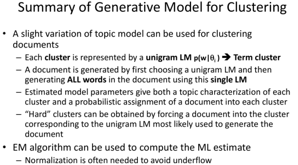
3.Text Clustering: Similarity-based Clustering 

 3.1 Similarity-based Clustering: General Idea

• Explicitly define a similarity function to measure similarity between two text objects (i.e., providing “clustering bias”)

• Find an optimal partitioning of data to

• • maximize intra-group similarity and
  • minimize inter-group similarity

• Two strategies for obtaining optimal clustering
•  Progressively construct a hierarchy of clusters (hierarchical clustering) 

• Bottom-up (agglomerative): gradually group similar objects into larger clusters
•  Top-down (divisive): gradually partition the data into smaller clusters

• Start with an initial tentative clustering and iteratively improve it (“flat”clustering, e.g., k-Means)

3.2 How does hierarchical agglomerative clustering work?

• Given a similarity function to measure similarity between two objects
• Gradually group similar objects together in a bottom-up fashion to form a hierarchy
• Stop when some stopping criterion is met
• Variations: different ways to compute group similarity based on individual object similarity

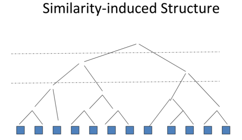
　　Start with all the text objects and we can then measure the similarity between them. Of course based on the provided similarity function, and then we can see which pair has the highest similarity. And then just group them together, and then we're going to see which pair is the next one to group.
Maybe these two now have the highest similarity, and then we're going to gradually group them together. And then every time we're going to pick the highest similarity, the similarity of pairs to group. This will give us a binary tree eventually to group everything together. 
　　Now, depending on our applications, we can use the whole hierarchy as a structure for browsing, for example. Or we can choose a cutoff, let's say cut here to get four clusters, or we can use a threshold to cut. Or we can cut at this high level to get just two clusters, so this is a general idea, now if you think about how to implement this algorithm. You'll realize that we have everything specified except for how to compute group similarity.

3.3 How to Compute Group Similarity

　　Three popular methods:

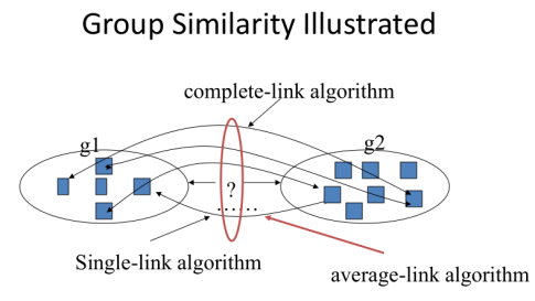
　　Given two groups g1 and g2,

• Single-link algorithm: s(g1,g2)= similarity of the closest pair

• Complete-link algorithm: s(g1,g2)= similarity of the farthest pair

• Average-link algorithm: s(g1,g2)= average of similarity of all pairs

　　Comparison of Single-Link, Complete-Link, and Average-Link:

　　①Single-link

•  “Loose” clusters
• Individual decision, sensitive to outliers

　　②Complete-link

• “Tight” clusters
• Individual decision, sensitive to outliers

　　③ Average-link

• “In between”
• Group decision, insensitive to outliers　

　　First, single-link can be expected to generally the loose clusters, the reason is because as long as two objects are very similar in the two groups, it will bring the two groups together. If you think about this as similar to having parties with people, then it just means two groups of people would be partying together. As long as in each group there is a person that is well connected with the other group. So the two leaders of the two groups can have a good relationship with each other and then they will bring together the two groups. In this case, the cluster is loose, because there's no guarantee that other members of the two groups are actually very close to each other. Sometimes they may be very far away, now in this case it's also based on individual decisions, so it could be sensitive to outliers.
　　The complete-link is in the opposite situation, where we can expect the clusters to be tight. And it's also based on individual decision so it can be sensitive to outliers. Again to continue the analogy to having a party of people, then complete-link would mean when two groups come together. They want to ensure that even the people that are unlikely to talk to each other would be comfortable. Always talking to each other, so ensure the whole class to be coherent.
　　The average link of clusters in between and as group decision, so it's going to be insensitive to outliers, now in practice which one is the best. Well, this would depend on the application and sometimes you need a lose clusters. And aggressively cluster objects together that maybe single-link is good. But other times you might need a tight clusters and a complete-link might be better. But in general, you have to empirically evaluate these methods for your application to know which one is better.

3.4 How does K-Means Clustering work？

• Represent each text object as a term vector and assume a similarity function defined on two objects
• Start with k randomly selected vectors and assume they are the centroids of k clusters (initial tentative clustering)
• Assign every vector to a cluster whose centroid is the closest to the vector
• Re-compute the centroid for each cluster based on the newly assigned vectors in the cluster
• Repeat this process until the similarity-based objective function (i.e., within cluster sum of squares) converges (to a local minimum)

　　It's very similar to clustering with EM for mixture model!

　　

　　Now let me summarize our discussion of clustering methods:

　　

4.Text Clustering:Evaluation

4.1 Direct Evaluation of Text Clusters

• Question to answer: How close are the system-generated clusters to the ideal clusters (generated by humans)?
• “Closeness” can be assessed from multiple perspectives
• “Closeness” can be quantified
• “Clustering bias” is imposed by the human assessors
• Evaluation procedure:
• Given a test set, have humans to create an ideal clustering result (i.e.,an ideal partitioning of text objects or “gold standard”)
• Use a system to produce clusters from the same test set
• Quantify the similarity between the system-generated clusters and the gold standard clusters
• Similarity can be measured from multiple perspectives (e.g., purity, normalized mutual information, F measure)

4.2 Indirect Evaluation of Text Clusters

• Question to answer: how useful are the clustering results for the intended applications?
• “Usefulness” is inevitably application specific
• “Clustering bias” is imposed by the intended application
• Evaluation procedure:
• Create a test set for the intended application to quantify the performance of any system for this application
• Choose a baseline system to compare with
• Add a clustering algorithm to the baseline system“clustering system”
• Compare the performance of the clustering system and the baseline in terms of any performance measure for the application

　　we call it indirect evaluation of clusters because there's no explicit assessment of the quality of clusters, but rather it's to assess the contribution of clusters to a particular application.

4.3 Summary of Text Clustering

• Text clustering is an unsupervised general text mining technique to
• obtain an overall picture of the text content (exploring text data)
• discover interesting clustering structures in text data
• Many approaches are possible
• Strong clusters tend to show up no matter what method used
• Effectiveness of a method highly depends on whether the desired clustering bias is captured appropriately (either through using the right generative model or the right similarity function)
• Deciding the optimal number of clusters is generally a difficult problem for any method due to the unsupervised nature
• Evaluation of clustering results can be done both directly and indirectly

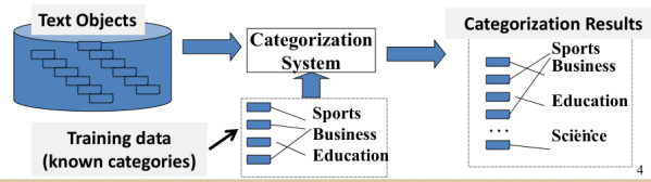
5.Text Categorization:Motivation

5.1 What is text categorization?

• Given the following:
• A set of predefined categories, possibly forming a hierarchy and often
• A training set of labeled text objects
• Task: Classify a text object into one or more of the categories

　　So, the problem of text categorization is defined as follows. We're given a set of predefined categories possibly forming a hierarchy or so. And often, also a set of training examples or training set of labeled text objects which means the text objects have already been enabled with known categories. And then, the task is to classify any text object into one or more of these predefined categories. 

 

5.2 What are some applications of text categorization?

　　Examples of Text Categorization:

• Text objects can vary (e.g., documents, passages, or collections of text)
• Categories can also vary
• “Internal” categories that characterize a text object (e.g., topical categories, sentiment categories)
• “External” categories that characterize an entity associated with the text object (e.g., author attribution or any other meaningful categories associated with text data)
• Some examples of applications
• News categorization, literature article categorization (e.g., MeSH annotations)
• Spam email detection/filtering
• Sentiment categorization of product reviews or tweets
• Automatic email sorting/routing
• Author attribution

　Variants of Problem Formulation:

• Binary categorization: Only two categories
• Retrieval: {relevant-doc, non-relevant-doc}
• Spam filtering: {spam, non-spam}
• Opinion: {positive, negative}
• K-category categorization: More than two categories
• Topic categorization: {sports, science, travel, business,…}
• Email routing: {folder1, folder2, folder3,…}
• Hierarchical categorization: Categories form a hierarchy
• Joint categorization: Multiple related categorization tasks done in a joint manner

　　Binary categorization can potentially support all other categorizations!

5.3 Why we use text categorization?

• To enrich text representation (more understanding of text)
• Text can now be represented in multiple levels (keywords + categories)
• Semantic categories assigned can be directly or indirectly useful for an application
• Semantic categories facilitate aggregation of text content (e.g., aggregating all positive/negative opinions about a product)
• To infer properties of entities associated with text data (discovery of knowledge about the world)
• As long as an entity can be associated with text data, we can always use the text data to help categorize the associated entities
• E.g., discovery of non-native speakers of a language; prediction of party affiliation based on a political speech

6.Text Categorization:Methods

6.1 Categorization Methods: Manual & “Automatic”

　　Manual:

• Determine the category based on rules that are carefully designed to reflect the domain knowledge about the categorization problem
• Works well when
• The categories are very well defined
• Categories are easily distinguished based on surface features in text (e.g., special vocabulary is known to only occur in a particular category)
• Sufficient domain knowledge is available to suggest many effective rules
• Problems
• Labor intensivedoesn’t scale up well
• Can’t handle uncertainty in rules; rules may be inconsistent not robust
• Both problems can be solved/alleviated by using machine learning

　　It's actually very hard to have 100% correct rule. So for example you can say well, if it has game, sports, basketball Then for sure it's about sports. But one can also imagine some types of articles that mention these cures, but may not be exactly about sports or only marginally touching sports. The main topic could be another topic, a different topic than sports. So that's one disadvantage of this approach. And then finally, the rules maybe inconsistent and this would lead to robustness. More specifically, and sometimes, the results of categorization may be different that depending on which rule to be applied. So as in that case that you are facing uncertainty. And you will also have to decide an order of applying the rules, or combination of results that are contradictory. So all these are problems with this approach. And it turns out that both problems can be solved or alleviated by using machine learning. 

　　“Automatic”:

• Use human experts to
•  Annotate data sets with category labels  Training data
•  P rovide a set of features to represent each text object that can potentially provide a “clue” about the category
• Use machine learning to learn “soft rules” for categorization from the training data
•  Figure out which features are most useful for separating different categories
•  Optimally combine the features to minimize the errors of categorization on the training data
•  The trained classifier can then be applied to a new text object to predict the most likely category (that a human expert would assign to it)

　　So these machine learning methods are more automatic. But, I still put automatic in quotation marks because they are not really completely automatic cause it still require many work. More specifically we have to use a human experts to help in two ways. First the human experts must annotate data cells was category labels. And would tell the computer which documents should receive which categories. And this is called training data. 

6.2 Machine Learning for Text Categorization

• General setup: Learn a classifier f: XY
• Input: X = all text objects; Output: Y = all categories
• Learn a classifier function, f: XY, such that f(x)=y Y gives the correct category for x X (“correct” is based on the training data)
• All methods
• Rely on discriminative features of text objects to distinguish categories
• Combine multiple features in a weighted manner
• Adjust weights on features to minimize errors on the training data
• Different methods tend to vary in
• Their way of measuring the errors on the training data (may optimize a different objective/loss/cost function)
• Their way of combining features (e.g., linear vs. non-linear)

6.3 Generative vs. Discriminative Classifiers

• Generative classifiers (learn what the data “looks” like in each category)
• Attempt to model p(X,Y) = p(Y)p(X|Y) and compute p(Y|X) based on p(X|Y) and p(Y) by using Bayes Rule
• Objective function is likelihood, thus indirectly measuring training errors
• E.g., Naïve Bayes
• Discriminative classifiers (learn what features separate categories)
• Attempt to model p(Y|X) directly
• Objective function directly measures errors of categorization on training data
• E.g., Logistic Regression, Support Vector Machine (SVM), k-Nearest Neighbors (kNN)

7.Text Categorization:Generative probabilistic models

7.1 Document Clustering Revisited

　　Now, suppose d has L words represented as xi here. Now, how can you compute the probability that a particular topic word distribution zeta i has been used to generate this document? 

　　Which cluster does d belong to? Which θ_i was used to generate d?

 

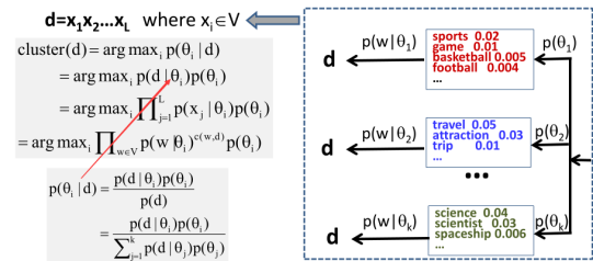
　　And we now can see clearly how we can assign a document to a category based on the information about word distributions for these categories and the prior on these categories. So this idea can be directly adapted to do categorization. And this is precisely what a Naive Bayes Classifier is doing. 

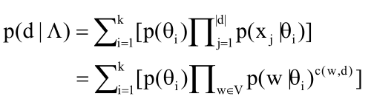
7.2 Text Categorization with Naïve Bayes Classifier

　　We assume that if theta i represents category i accurately, that means the word distribution characterizes the content of documents in category i accurately. Then, what we can do is precisely like what we did for text clustering. Namely we're going to assign document d to the category that has the highest probability of generating this document. In other words, we're going to maximize this posterior probability as well. 

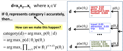
 　　So basically, with Naive Bayes Classifier, we're going to score each category for the document by this function. 

　　Now, you may notice that here it involves a product of a lot of small probabilities. So one way to solve the problem is thru take logarithm of this function, which it doesn't changes all the often these categories. But will helps us preserve precision. And so, this is often the function that we actually use to score each category and then we're going to choose the category that has the highest score by this function. So this is called an Naive Bayes Classifier, now the keyword base is understandable because we are applying a base rule here when we go from the posterior probability of the topic to a product of the likelihood and the prior. 

　　Now, it's also called a naive because we've made an assumption that every word in the document is generated independently, and this is indeed a naive assumption because in reality they're not generating independently. Once you see some word, then other words will more likely occur. For example, if you have seen a word like a text. Than that mixed category, they see more clustering more likely to appear than if you have not the same text. 

7.3 Learn from the Training Data

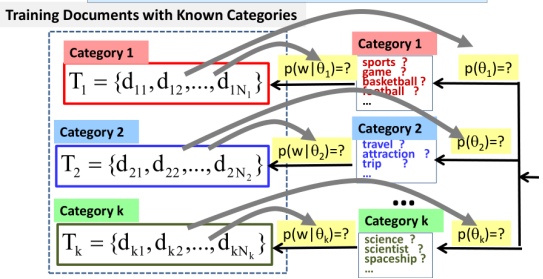
 　　Now the question is, how can we make sure theta i actually represents category i accurately? Well if you think about the question, and you likely come up with the idea of using the training data. 

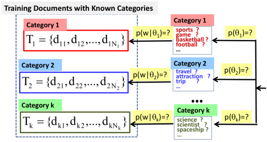
　　These are the documents with known categories assigned and of course human experts must do that. In here, you see that T1 represents the set of documents that are known to have the generator from category 1. And T2 represents the documents that are known to have been generated from category 2, etc. Now if you look at this picture, you'll see that the model here is really a simplified unigram language model. It's no longer mixed modal, why? Because we already know which distribution has been used to generate which documents. There's no uncertainty here, there's no mixing of different categories here.
So the estimation problem of course would be simplified. But in general, you can imagine what we want to do is estimate these probabilities that I marked here. And what other probability is that we have to estimate it in order to do relation. Well there are two kinds. So one is the prior, the probability of theta i and this indicates how popular each category is or how likely will it have observed the document in that category. The other kind is the water distributions and we want to know what words have high probabilities for each category. So the idea then is to just use observe the training data to estimate these two probabilities.

7.3 How to Estimate p(w|θ_i) and p(θ_i )

　　This is a statistical estimation problem. We have observed some data from some model and we want to guess the parameters of this model. We want to take our best guess of the parameters. 

　　 Let's just think about with category 1, we know there is one word of distribution that has been used to generate documents. And we generate each word in the document independently, and we know that we have observed a set of n sub 1 documents in the set of Q1. These documents have been all generated from category 1. Namely have been all generated using this same word distribution. Now the question is, what would be your guess or estimate of the probability of each word in this distribution? And what would be your guess of the entire probability of this category? Of course, this singular probability depends on how likely are you to see documents in other categories? 

　　First, what's the bases for estimating the prior or the probability of each category. And what about the basis for estimating the probability of where each category? Well the same, and you'll be just assuming that words that are observed frequently in the documents that are known to be generated from a category will likely have a higher probability. And that's just a maximum Naive Bayes made of. Indeed, that's what we can do, so this made the probability of which category and to answer the question, which category is most popular? Then we can simply normalize, the count of documents in each category. So here you see N sub i denotes the number of documents in each category.
And we simply just normalize these counts to make this a probability. In other words, we make this probability proportional to the size of training intercept in each category that's a size of the set t sub i.

 

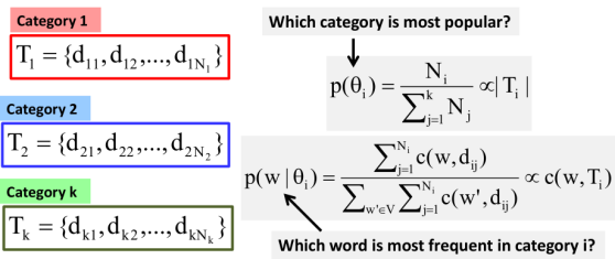
　　Now what about the word distribution? Well, we do the same. Again this time we can do this for each category. So let's say, we're considering category i or theta i. So which word has a higher probability? Well, we simply count the word occurrences in the documents that are known to be generated from theta i. And then we put together all the counts of the same word in the set. And then we just normalize these counts to make this distribution of all the words make all the probabilities off these words to 1. So in this case, you're going to see this is a proportional through the count of the word in the collection of training documents T sub i and that's denoted by c of w and T sub i.

7.4 Smoothing in Naïve Bayes 

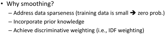
 　　There is another issue in Naive Bayes which is a smoothing. In fact the smoothing is a general problem in older estimate of language morals. And this has to do with, what would happen if you have observed a small amount of data? So smoothing is an important technique to address that outsmarts this. In our case, the training data can be small and when the data set is small when we use maximum likely estimator we often face the problem of zero probability. That means if an event is not observed then the estimated probability would be zero. In this case, if we have not seen a word in the training documents for let's say, category i. Then our estimator would be zero for the probability of this one in this category, and this is generally not accurate. So we have to do smoothing to make sure it's not zero probability. The other reason for smoothing is that this is a way to bring prior knowledge, and this is also generally true for a lot of situations of smoothing. When the data set is small, we tend to rely on some prior knowledge to solve the problem.  So smoothing allows us to inject these to prior initial that no order has a real zero probability.There is also a third reason which us sometimes not very obvious. And that is to help achieve discriminative weighting of terms. And this is also called IDF weighting, inverse document frequency weighting that you have seen in mining word relations. 

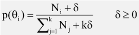
　　So how do we do smoothing? Well in general we add pseudo counts to these events, we'll make sure that no event has 0 count. So one possible way of smoothing the probability of the category is to simply add a small non active constant delta to the count. Let's pretend that every category has actually some extra number of documents represented by delta. And in the denominator we also add a k multiplied by delta because we want the probability to some to 1. So in total we've added delta k times because we have a k categories. Therefore in this sum, we have to also add k multiply by delta as a total pseudocount that we add up to the estimate. 

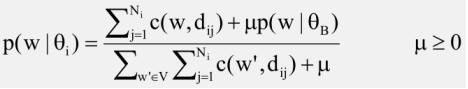
　　So in general, in Naive Bayes categorization we have to do such a small thing. And then once we have these probabilities, then we can compute the score for each category. 

7.5 Anatomy of Naïve Bayes Classifier

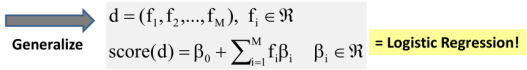
　　Lets say this is our scoring function for two categories. So, this is a score of a document for these two categories. And we're going to score based on this probability ratio. So if the ratio is larger, then it means it's more likely to be in category one. So the larger the score is the more likely the document is in category one. 

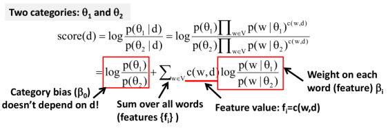
　　And with a proper setting of the weights, then we can expect such a scoring function to work well to classify documents, just like in the case of naive Bayes. We can clearly see naive Bayes classifier as a special case of this general classifier. Actually, this general form is very close to a classifier called a logistical regression, and this is actually one of those conditional approaches or discriminative approaches to classification.