BP神经网络求解异或问题(Python实现)

反向传播算法(Back Propagation)分二步进行，即正向传播和反向传播。这两个过程简述如下：

1．正向传播

输入的样本从输入层经过隐单元一层一层进行处理，传向输出层；在逐层处理的过程中。在输出层把当前输出和期望输出进行比较，如果现行输出不等于期望输出，则进入反向传播过程。

2．反向传播

反向传播时，把误差信号按原来正向传播的通路反向传回，逐层修改连接权值，以望代价函数趋向最小。

下面以单隐层的神经网络为例，进行权值调整的公式推导，其结构示意图如下：

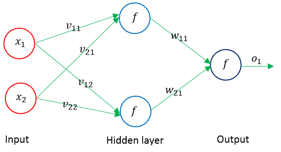
输入层输入向量(n维)：X=(x1,x2,…,xi,…,xn)T

隐层输出向量(隐层有m个结点)：Y=(y1,y2,…,yj,…,ym)T

输出层输出向量(l维)：O=(o1,o2,…,ok,…,ol)T

期望输出向量：d=(d1, d2,…,dk,…,dl)T

输入层到隐层之间的权值矩阵：V=(V1,V2,…,Vj,…,Vm)

隐层到输出层之间的权值矩阵用：W=(W1,W2,…,Wk,…,Wl)

对输出层第k个结点和隐含层的第j个结点有如下关系：

激活函数f(x)常用sigmoid函数(一个在生物学中常见的S型的函数，也称为S形生长曲线)或者tanh(双曲正切)函数。各种S型曲线函数如下图所示：

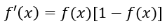
下面以sigmoid函数进行推导。sigmoid函数定义为：

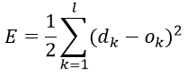
其导函数为：

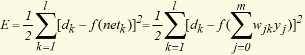
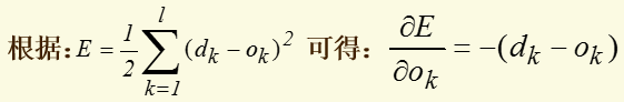
定义对单个样本输出层所有神经元的误差总能量总和为：

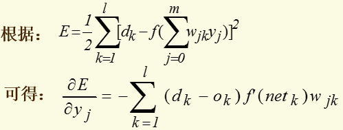
将以上误差定义式展开至隐层：

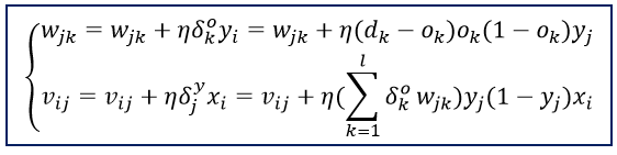
权值调整思路为：

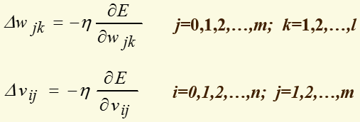
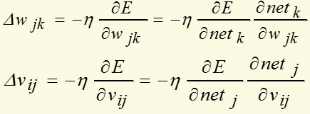
上面式子中负号表示梯度下降，常数η∈(0,1)表示权值调整步长(学习速度)。推导过程中，对输出层有j=0,1,2,…,m;  k=1,2,…,l；对隐层有 i=0,1,2,…,n;  j=1,2,…,m

对输出层和隐层，上面式子可写为：

对输出层和隐层，定义δ：

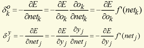
将以上结果代入δ的表达式，并根据sigmoid函数与其导函数的关系:f'(x)=f(x)*[1-f(x)],可以计算出：

 

可以看出要计算隐层的δ，需要先从输出层开始计算，显然它是反向递推计算的公式。以此类推，对于多层神经网络，要先计算出最后一层(输出层)的δ，然后再递推计算前一层，直到输入层。根据上述结果，三层前馈网的BP学习算法权值调整计算公式为：

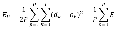
对所有输入样本(P为训练样本的个数)，以总的平均误差能量作为经验损失函数（经验风险函数，代价函数）为：

最终目标是需要调整连接权使得经验损失函数最小。用BP算法训练网络时有两种训练方式：一种是顺序方式(Stochastic Learning)，即每输入一个训练么样本修改一次权值；以上给出的权值修正步骤就是按顺序方式训练网络的；另一种是批处理方式(Batch Learning)，即待组成一个训练周期的全部样本都一次输入网络后，以Ep为目标函数修正权值.

顺序方式所需的临时存储空间较批处理方式小，而且随机输入样本有利于权值空间的搜索具有随机性，在一定程度上可以避免学习陷入局部最小值。但是顺序方式的误差收敛条件难以建立，而批处理方式能精确地计算出梯度向量，误差收敛条件简单。

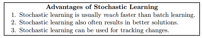
Stochastic learning is generally the preferred method for basic backpropagation for the following three reasons：

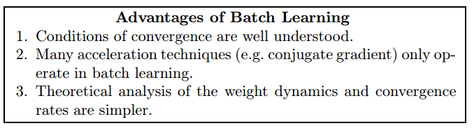
Despite the advantages of stochastic learning, there are still reasons why one might consider using batch learning:

 

下面采用激活函数为tanh(x)的三层网络来解决异或问题(当激活函数为奇函数时,BP 算法的学习速度要快一些，最常用的奇函数是双曲正切函数)

# -*- coding: utf-8 -*-
import numpy as np


# 双曲正切函数,该函数为奇函数
def tanh(x):    
    return np.tanh(x)

# tanh导函数性质:f'(t) = 1 - f(x)^2
def tanh_prime(x):      
    return 1.0 - tanh(x)**2


class NeuralNetwork:
    def __init__(self, layers, activation = 'tanh'):
        """
        :参数layers: 神经网络的结构(输入层-隐含层-输出层包含的结点数列表)
        :参数activation: 激活函数类型
        """
        if activation == 'tanh':    # 也可以用其它的激活函数
            self.activation = tanh
            self.activation_prime = tanh_prime
        else:
            pass

        # 存储权值矩阵
        self.weights = []

        # range of weight values (-1,1)
        # 初始化输入层和隐含层之间的权值
        for i in range(1, len(layers) - 1):
            r = 2*np.random.random((layers[i-1] + 1, layers[i] + 1)) -1     # add 1 for bias node
            self.weights.append(r)
            
        # 初始化输出层权值
        r = 2*np.random.random( (layers[i] + 1, layers[i+1])) - 1         
        self.weights.append(r)


    def fit(self, X, Y, learning_rate=0.2, epochs=10000):
        # Add column of ones to X
        # This is to add the bias unit to the input layer
        X = np.hstack([np.ones((X.shape[0],1)),X])
     
        
        for k in range(epochs):     # 训练固定次数
            if k % 1000 == 0: print 'epochs:', k

            # Return random integers from the discrete uniform distribution in the interval [0, low).
            i = np.random.randint(X.shape[0],high=None) 
            a = [X[i]]   # 从m个输入样本中随机选一组

            for l in range(len(self.weights)): 
                    dot_value = np.dot(a[l], self.weights[l])   # 权值矩阵中每一列代表该层中的一个结点与上一层所有结点之间的权值
                    activation = self.activation(dot_value)
                    a.append(activation)
                    
            # 反向递推计算delta:从输出层开始,先算出该层的delta,再向前计算
            error = Y[i] - a[-1]    # 计算输出层delta
            deltas = [error * self.activation_prime(a[-1])]
            
            # 从倒数第2层开始反向计算delta
            for l in range(len(a) - 2, 0, -1): 
                deltas.append(deltas[-1].dot(self.weights[l].T)*self.activation_prime(a[l]))


            # [level3(output)->level2(hidden)]  => [level2(hidden)->level3(output)]
            deltas.reverse()    # 逆转列表中的元素


            # backpropagation
            # 1. Multiply its output delta and input activation to get the gradient of the weight.
            # 2. Subtract a ratio (percentage) of the gradient from the weight.
            for i in range(len(self.weights)):  # 逐层调整权值
                layer = np.atleast_2d(a[i])     # View inputs as arrays with at least two dimensions
                delta = np.atleast_2d(deltas[i])
                self.weights[i] += learning_rate * np.dot(layer.T, delta) # 每输入一次样本,就更新一次权值

    def predict(self, x): 
        a = np.concatenate((np.ones(1), np.array(x)))       # a为输入向量(行向量)
        for l in range(0, len(self.weights)):               # 逐层计算输出
            a = self.activation(np.dot(a, self.weights[l]))
        return a



if __name__ == '__main__':
    nn = NeuralNetwork([2,2,1])     # 网络结构: 2输入1输出,1个隐含层(包含2个结点)

    X = np.array([[0, 0],           # 输入矩阵(每行代表一个样本,每列代表一个特征)
                  [0, 1],
                  [1, 0],
                  [1, 1]])
    Y = np.array([0, 1, 1, 0])      # 期望输出

    nn.fit(X, Y)                    # 训练网络

    print 'w:', nn.weights          # 调整后的权值列表
    
    for s in X:
        print(s, nn.predict(s))     # 测试

输出为：

参考：

http://www.bogotobogo.com/python/python_Neural_Networks_Backpropagation_for_XOR_using_one_hidden_layer.php

https://triangleinequality.wordpress.com/2014/03/31/neural-networks-part-2/

https://databoys.github.io/Feedforward/

http://www.cnblogs.com/wentingtu/archive/2012/06/05/2536425.html

《Neural Networks Tricks of the Trade》Second Edition