mysql 索引 聚簇索引 聚集索引 非聚集索引 clustered indexes nonclustered InnoDB 索引组织表 Index Organizied Table 堆组织表Heap Organizied Table
聚集索引和非聚集索引在索引结构中都只包含键和记录标识符。记录标识符总是指向数据页中的行。
使用聚集索引,数据库管理器将尝试以与索引页中相应键相同的顺序保持数据页中的数据。
因此,数据库管理器尝试将具有相似键的行插入到相同的页面上。如果对表进行了重组,则按照索引键的顺序将数据插入数据页。与非聚集索引的对应键的顺序相比,数据库管理器不维护数据的任何顺序。
Clustered and non-clustered indexes - IBM Documentation https://www.ibm.com/docs/en/ias?topic=indexes-clustered-non-clustered
Clustered and non-clustered indexes
Last Updated: 2022-10-04
Index architectures are classified as clustered or non-clustered. Clustered indexes are indexes whose order of the rows in the data pages corresponds to the order of the rows in the index. This order is why only one clustered index can exist in any table, whereas, many non-clustered indexes can exist in the table. In some database systems, the leaf node of the clustered index corresponds to the actual data, not a pointer to data that is found elsewhere.
Both clustered and non-clustered indexes contain only keys and record identifiers in the index structure. The record identifiers always point to rows in the data pages. With clustered indexes, the database manager attempts to keep the data in the data pages in the same order as the corresponding keys in the index pages. Thus the database manager attempts to insert rows with similar keys onto the same pages. If the table is reorganized, data is inserted into the data pages in the order of the index keys. The database manager does not maintain any order of the data when compared to the order of the corresponding keys of a non-clustered index.
Reorganizing a table with a chosen index reclusters the data. A clustered index is most useful for columns that have range predicates because it allows better sequential access of data in the table. As a result, since like values are on the same data page, fewer pages are fetched.
In general, only one of the indexes in a table can have a high degree of clustering.
Clustering indexes can improve the performance of most query operations because they provide a more linear access path to data, which is stored in pages. In addition, because rows with similar index key values are stored together, sequential detection prefetching is more efficient when clustering indexes are used.
Improving performance with clustering indexes
Generally, clustering is more effectively maintained if the clustering index is unique.
Clustered and nonclustered indexes described - SQL Server | Microsoft Learn https://learn.microsoft.com/en-us/sql/relational-databases/indexes/clustered-and-nonclustered-indexes-described?view=sql-server-ver16
描述的聚集索引和非聚集索引 - SQL Server | Microsoft Learn https://learn.microsoft.com/zh-cn/sql/relational-databases/indexes/clustered-and-nonclustered-indexes-described?view=sql-server-ver16
索引是与表或视图关联的磁盘上结构,可以加快从表或视图中检索行的速度。 索引包含由表或视图中的一列或多列生成的键。 这些键存储在一个结构(B 树)中,使 SQL Server 可以快速有效地查找与键值关联的行。
备注
SQL Server 文档在提到索引时一般使用 B 树这个术语。 在行存储索引中,SQL Server 实现了 B+ 树。 这不适用于列存储索引或内存中数据存储。 有关详细信息,请参阅SQL Server和Azure SQL索引体系结构和设计指南。
表或视图可以包含以下类型的索引:
-
聚集
- 聚集索引根据数据行的键值在表或视图中排序和存储这些数据行。 索引定义中包含聚集索引列。 每个表只能有一个聚集索引,因为数据行本身只能按一个顺序存储。
- 只有当表包含聚集索引时,表中的数据行才按排序顺序存储。 如果表具有聚集索引,则该表称为聚集表。 如果表没有聚集索引,则其数据行存储在一个称为堆的无序结构中。
-
非聚集
-
非聚集索引具有独立于数据行的结构。 非聚集索引包含非聚集索引键值,并且每个键值项都有指向包含该键值的数据行的指针。
-
从非聚集索引中的索引行指向数据行的指针称为行定位器。 行定位器的结构取决于数据页是存储在堆中还是聚集表中。 对于堆,行定位器是指向行的指针。 对于聚集表,行定位器是聚集索引键。
-
可以向非聚集索引的叶级添加非键列以跳过现有的索引键限制,并执行完整范围内的索引查询。 有关详细信息,请参阅创建带有包含列的索引。 有关索引键限制的详细信息,请参阅 SQL Server 的最大容量规范。
-
聚集索引和非聚集索引都可以是唯一的。 这意味着任何两行都不能有相同的索引键值。 另外,索引也可以不是唯一的,即多行可以共享同一键值。 有关详细信息,请参阅创建唯一索引。
每当修改了表数据后,都会自动维护表或视图的索引。
有关其他类型的特殊用途索引,请参阅 Indexes 。
索引和约束
对表列定义了 PRIMARY KEY 约束和 UNIQUE 约束时,会自动创建索引。 例如,在创建带 UNIQUE 约束的表时,数据库引擎 自动创建非聚集索引。 如果你配置 PRIMARY KEY,数据库引擎 会自动创建聚集索引(除非聚集索引已存在)。 如果你尝试对现有表强制执行 PRIMARY KEY 约束,且此表上已有聚集索引,SQL Server 使用非聚集索引强制执行主键。
查询优化器如何使用索引
设计良好的索引可以减少磁盘 I/O 操作,并且消耗的系统资源也较少,从而可以提高查询性能。 对于包含 SELECT、UPDATE、DELETE 或 MERGE 语句的各种查询,索引会很有用。 例如,在 SELECT Title, HireDate FROM HumanResources.Employee WHERE EmployeeID = 250 数据库中执行的查询 AdventureWorks2022 。 执行此查询时,查询优化器评估可用于检索数据的每个方法,然后选择最有效的方法。 可能采用的方法包括扫描表和扫描一个或多个索引(如果有)。
扫描表时,查询优化器读取表中的所有行,并提取满足查询条件的行。 扫描表会有许多磁盘 I/O 操作,并占用大量资源。 但是,如果查询的结果集是占表中较高百分比的行,扫描表会是最为有效的方法。
查询优化器使用索引时,搜索索引键列,查找到查询所需行的存储位置,然后从该位置提取匹配行。 通常,搜索索引比搜索表要快很多,因为索引与表不同,一般每行包含的列非常少,且行遵循排序顺序。
查询优化器在执行查询时通常会选择最有效的方法。 但如果没有索引,则查询优化器必须扫描表。 您的任务是设计并创建最适合您的环境的索引,以便查询优化器可以从多个有效的索引中选择。 SQL Server 提供 数据库引擎优化顾问 以帮助分析数据库环境并选择适当的索引。
An index is an on-disk structure associated with a table or view that speeds retrieval of rows from the table or view. An index contains keys built from one or more columns in the table or view. These keys are stored in a structure (B-tree) that enables SQL Server to find the row or rows associated with the key values quickly and efficiently.
Note
SQL Server documentation uses the term B-tree generally in reference to indexes. In rowstore indexes, SQL Server implements a B+ tree. This does not apply to columnstore indexes or in-memory data stores. For more information, see the SQL Server and Azure SQL index architecture and design guide.
A table or view can contain the following types of indexes:
-
Clustered
- Clustered indexes sort and store the data rows in the table or view based on their key values. These are the columns included in the index definition. There can be only one clustered index per table, because the data rows themselves can be stored in only one order.
- The only time the data rows in a table are stored in sorted order is when the table contains a clustered index. When a table has a clustered index, the table is called a clustered table. If a table has no clustered index, its data rows are stored in an unordered structure called a heap.
-
Nonclustered
-
Nonclustered indexes have a structure separate from the data rows. A nonclustered index contains the nonclustered index key values and each key value entry has a pointer to the data row that contains the key value.
-
The pointer from an index row in a nonclustered index to a data row is called a row locator. The structure of the row locator depends on whether the data pages are stored in a heap or a clustered table. For a heap, a row locator is a pointer to the row. For a clustered table, the row locator is the clustered index key.
-
You can add nonkey columns to the leaf level of the nonclustered index to by-pass existing index key limits, and execute fully covered, indexed, queries. For more information, see Create indexes with included columns. For details about index key limits see Maximum capacity specifications for SQL Server.
-
Both clustered and nonclustered indexes can be unique. This means no two rows can have the same value for the index key. Otherwise, the index is not unique and multiple rows can share the same key value. For more information, see Create unique indexes.
Indexes are automatically maintained for a table or view whenever the table data is modified.
See Indexes for additional types of special purpose indexes.
Indexes and constraints
Indexes are automatically created when PRIMARY KEY and UNIQUE constraints are defined on table columns. For example, when you create a table with a UNIQUE constraint, Database Engine automatically creates a nonclustered index. If you configure a PRIMARY KEY, Database Engine automatically creates a clustered index, unless a clustered index already exists. When you try to enforce a PRIMARY KEY constraint on an existing table and a clustered index already exists on that table, SQL Server enforces the primary key using a nonclustered index.
For more information, see Create primary keys and Create unique constraints.
How indexes are used by the Query Optimizer
Well-designed indexes can reduce disk I/O operations and consume fewer system resources therefore improving query performance. Indexes can be helpful for a variety of queries that contain SELECT, UPDATE, DELETE, or MERGE statements. Consider the query SELECT Title, HireDate FROM HumanResources.Employee WHERE EmployeeID = 250 in the AdventureWorks2022 database. When this query is executed, the query optimizer evaluates each available method for retrieving the data and selects the most efficient method. The method may be a table scan, or may be scanning one or more indexes if they exist.
When performing a table scan, the query optimizer reads all the rows in the table, and extracts the rows that meet the criteria of the query. A table scan generates many disk I/O operations and can be resource intensive. However, a table scan could be the most efficient method if, for example, the result set of the query is a high percentage of rows from the table.
When the query optimizer uses an index, it searches the index key columns, finds the storage location of the rows needed by the query and extracts the matching rows from that location. Generally, searching the index is much faster than searching the table because unlike a table, an index frequently contains very few columns per row and the rows are in sorted order.
The query optimizer typically selects the most efficient method when executing queries. However, if no indexes are available, the query optimizer must use a table scan. Your task is to design and create indexes that are best suited to your environment so that the query optimizer has a selection of efficient indexes from which to select. SQL Server provides the Database Engine Tuning Advisor to help with the analysis of your database environment and in the selection of appropriate indexes.
CREATE TABLE t1(id INT PRIMARY KEY, c INT) ENGINE=Memory;
CREATE TABLE t2(id INT PRIMARY KEY, c INT) ENGINE=InnoDB;
INSERT INTO t1 VALUES(1,1),(2,2),(3,3),(4,4),(5,5),(6,6),(7,7),(8,8),(9,9),(0,0);
INSERT INTO t2 VALUES(1,1),(2,2),(3,3),(4,4),(5,5),(6,6),(7,7),(8,8),(9,9),(0,0);
SELECT * FROM t1;
SELECT * FROM t2;

InnoDB表的数据就放在主键索引树上,主键索引是B+树。所以表t2的数据组织方式如下图所示:

Memory引擎的数据和索引是分开的

可以看到,内存表的数据部分以数组的方式单独存放,而主键id索引里,存的是每个数据的位置。主键id是hash索引,可以看到索引上的key并不是有序的。
在内存表t1中,当我执行select *的时候,走的是全表扫描,也就是顺序扫描这个数组。因此,0就是最后一个被读到,并放入结果集的数据。
可见,InnoDB和Memory引擎的数据组织方式是不同的:
- InnoDB引擎把数据放在主键索引上,其他索引上保存的是主键id。这种方式,我们称之为索引组织表(Index Organizied Table)。
- 而Memory引擎采用的是把数据单独存放,索引上保存数据位置的数据组织形式,我们称之为堆组织表(Heap Organizied Table)。
从中我们可以看出,这两个引擎的一些典型不同:
-
InnoDB表的数据总是有序存放的,而内存表的数据就是按照写入顺序存放的;
-
当数据文件有空洞的时候,InnoDB表在插入新数据的时候,为了保证数据有序性,只能在固定的位置写入新值,而内存表找到空位就可以插入新值;
-
数据位置发生变化的时候,InnoDB表只需要修改主键索引,而内存表需要修改所有索引;
-
InnoDB表用主键索引查询时需要走一次索引查找,用普通索引查询的时候,需要走两次索引查找。而内存表没有这个区别,所有索引的“地位”都是相同的。
-
InnoDB支持变长数据类型,不同记录的长度可能不同;内存表不支持Blob 和 Text字段,并且即使定义了varchar(N),实际也当作char(N),也就是固定长度字符串来存储,因此内存表的每行数据长度相同。
由于内存表的这些特性,每个数据行被删除以后,空出的这个位置都可以被接下来要插入的数据复用。比如,如果要在表t1中执行:
DELETE FROM t1 WHERE id=5;
INSERT INTO t1 VALUES(10,10);
SELECT * FROM t1;

explain SELECT * FROM t1 WHERE id<5;
explain SELECT * FROM t2 WHERE id<5;

mysql> explain SELECT * FROM t1 WHERE id<5;
+----+-------------+-------+------------+------+---------------+------+---------+------+------+----------+-------------+
| id | select_type | table | partitions | type | possible_keys | key | key_len | ref | rows | filtered | Extra |
+----+-------------+-------+------------+------+---------------+------+---------+------+------+----------+-------------+
| 1 | SIMPLE | t1 | NULL | ALL | PRIMARY | NULL | NULL | NULL | 10 | 33.33 | Using where |
+----+-------------+-------+------------+------+---------------+------+---------+------+------+----------+-------------+
1 row in set, 1 warning (0.00 sec)
mysql> explain SELECT * FROM t2 WHERE id<5;
+----+-------------+-------+------------+-------+---------------+---------+---------+------+------+----------+-------------+
| id | select_type | table | partitions | type | possible_keys | key | key_len | ref | rows | filtered | Extra |
+----+-------------+-------+------------+-------+---------------+---------+---------+------+------+----------+-------------+
| 1 | SIMPLE | t2 | NULL | range | PRIMARY | PRIMARY | 4 | NULL | 5 | 100.00 | Using where |
+----+-------------+-------+------------+-------+---------------+---------+---------+------+------+----------+-------------+
1 row in set, 1 warning (0.00 sec)
mysql>
38讲都说InnoDB好,那还要不要使用Memory引擎
https://funnylog.gitee.io/mysql45/38%E8%AE%B2%E9%83%BD%E8%AF%B4InnoDB%E5%A5%BD%EF%BC%8C%E9%82%A3%E8%BF%98%E8%A6%81%E4%B8%8D%E8%A6%81%E4%BD%BF%E7%94%A8Memory%E5%BC%95%E6%93%8E.html
mysql 索引 聚簇索引
剖析Mysql的InnoDB索引_voidccc的博客-CSDN博客 https://blog.csdn.net/voidccc/article/details/40077329
剖析Mysql的InnoDB索引
voidccc
摘要:
本篇介绍下Mysql的InnoDB索引相关知识,从各种树到索引原理到存储的细节。
InnoDB是Mysql的默认存储引擎(Mysql5.5.5之前是MyISAM,文档)。本着高效学习的目的,本篇以介绍InnoDB为主,少量涉及MyISAM作为对比。
这篇文章是我在学习过程中总结完成的,内容主要来自书本和博客(参考文献会给出),过程中加入了一些自己的理解,描述不准确的地方烦请指出。
1 各种树形结构
本来不打算从二叉搜索树开始,因为网上已经有太多相关文章,但是考虑到清晰的图示对理解问题有很大帮助,也为了保证文章完整性,最后还是加上了这部分。
先看看几种树形结构:
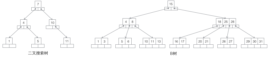
1 搜索二叉树:每个节点有两个子节点,数据量的增大必然导致高度的快速增加,显然这个不适合作为大量数据存储的基础结构。
2 B树:一棵m阶B树是一棵平衡的m路搜索树。最重要的性质是每个非根节点所包含的关键字个数 j 满足:┌m/2┐ - 1 <= j <= m - 1;一个节点的子节点数量会比关键字个数多1,这样关键字就变成了子节点的分割标志。一般会在图示中把关键字画到子节点中间,非常形象,也容易和后面的B+树区分。由于数据同时存在于叶子节点和非叶子结点中,无法简单完成按顺序遍历B树中的关键字,必须用中序遍历的方法。
3 B+树:一棵m阶B树是一棵平衡的m路搜索树。最重要的性质是每个非根节点所包含的关键字个数 j 满足:┌m/2┐ - 1 <= j <= m;子树的个数最多可以与关键字一样多。非叶节点存储的是子树里最小的关键字。同时数据节点只存在于叶子节点中,且叶子节点间增加了横向的指针,这样顺序遍历所有数据将变得非常容易。
4 B*树:一棵m阶B树是一棵平衡的m路搜索树。最重要的两个性质是1每个非根节点所包含的关键字个数 j 满足:┌m2/3┐ - 1 <= j <= m;2非叶节点间添加了横向指针。


B/B+/B*三种树有相似的操作,比如检索/插入/删除节点。这里只重点关注插入节点的情况,且只分析他们在当前节点已满情况下的插入操作,因为这个动作稍微复杂且能充分体现几种树的差异。与之对比的是检索节点比较容易实现,而删除节点只要完成与插入相反的过程即可(在实际应用中删除并不是插入的完全逆操作,往往只删除数据而保留下空间为后续使用)。
先看B树的分裂,下图的红色值即为每次新插入的节点。每当一个节点满后,就需要发生分裂(分裂是一个递归过程,参考下面7的插入导致了两层分裂),由于B树的非叶子节点同样保存了键值,所以已满节点分裂后的值将分布在三个地方:1原节点,2原节点的父节点,3原节点的新建兄弟节点(参考5,7的插入过程)。分裂有可能导致树的高度增加(参考3,7的插入过程),也可能不影响树的高度(参考5,6的插入过程)。

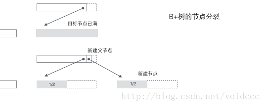
B+树的分裂:当一个结点满时,分配一个新的结点,并将原结点中1/2的数据复制到新结点,最后在父结点中增加新结点的指针;B+树的分裂只影响原结点和父结点,而不会影响兄弟结点,所以它不需要指向兄弟节点的指针。
B*树的分裂:当一个结点满时,如果它的下一个兄弟结点未满,那么将一部分数据移到兄弟结点中,再在原结点插入关键字,最后修改父结点中兄弟结点的关键字(因为兄弟结点的关键字范围改变了)。如果兄弟也满了,则在原结点与兄弟结点之间增加新结点,并各复制1/3的数据到新结点,最后在父结点增加新结点的指针。可以看到B*树的分裂非常巧妙,因为B*树要保证分裂后的节点还要2/3满,如果采用B+树的方法,只是简单的将已满的节点一分为二,会导致每个节点只有1/2满,这不满足B*树的要求了。所以B*树采取的策略是在本节点满后,继续插入兄弟节点(这也是为什么B*树需要在非叶子节点加一个兄弟间的链表),直到把兄弟节点也塞满,然后拉上兄弟节点一起凑份子,自己和兄弟节点各出资1/3成立新节点,这样的结果是3个节点刚好是2/3满,达到B*树的要求,皆大欢喜。

B+树适合作为数据库的基础结构,完全是因为计算机的内存-机械硬盘两层存储结构。内存可以完成快速的随机访问(随机访问即给出任意一个地址,要求返回这个地址存储的数据)但是容量较小。而硬盘的随机访问要经过机械动作(1磁头移动 2盘片转动),访问效率比内存低几个数量级,但是硬盘容量较大。典型的数据库容量大大超过可用内存大小,这就决定了在B+树中检索一条数据很可能要借助几次磁盘IO操作来完成。如下图所示:通常向下读取一个节点的动作可能会是一次磁盘IO操作,不过非叶节点通常会在初始阶段载入内存以加快访问速度。同时为提高在节点间横向遍历速度,真实数据库中可能会将图中蓝色的CPU计算/内存读取优化成二叉搜索树(InnoDB中的page directory机制)。

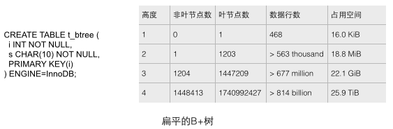
真实数据库中的B+树应该是非常扁平的,可以通过向表中顺序插入足够数据的方式来验证InnoDB中的B+树到底有多扁平。我们通过如下图的CREATE语句建立一个只有简单字段的测试表,然后不断添加数据来填充这个表。通过下图的统计数据(来源见参考文献1)可以分析出几个直观的结论,这几个结论宏观的展现了数据库里B+树的尺度。
1 每个叶子节点存储了468行数据,每个非叶子节点存储了大约1200个键值,这是一棵平衡的1200路搜索树!
2 对于一个22.1G容量的表,也只需要高度为3的B+树就能存储了,这个容量大概能满足很多应用的需要了。如果把高度增大到4,则B+树的存储容量立刻增大到25.9T之巨!
3 对于一个22.1G容量的表,B+树的高度是3,如果要把非叶节点全部加载到内存也只需要少于18.8M的内存(如何得出的这个结论?因为对于高度为2的树,1203个叶子节点也只需要18.8M空间,而22.1G从良表的高度是3,非叶节点1204个。同时我们假设叶子节点的尺寸是大于非叶节点的,因为叶子节点存储了行数据而非叶节点只有键和少量数据。),只使用如此少的内存就可以保证只需要一次磁盘IO操作就检索出所需的数据,效率是非常之高的。
2 Mysql的存储引擎和索引
可以说数据库必须有索引,没有索引则检索过程变成了顺序查找,O(n)的时间复杂度几乎是不能忍受的。我们非常容易想象出一个只有单关键字组成的表如何使用B+树进行索引,只要将关键字存储到树的节点即可。当数据库一条记录里包含多个字段时,一棵B+树就只能存储主键,如果检索的是非主键字段,则主键索引失去作用,又变成顺序查找了。这时应该在第二个要检索的列上建立第二套索引。 这个索引由独立的B+树来组织。有两种常见的方法可以解决多个B+树访问同一套表数据的问题,一种叫做聚簇索引(clustered index ),一种叫做非聚簇索引(secondary index)。这两个名字虽然都叫做索引,但这并不是一种单独的索引类型,而是一种数据存储方式。对于聚簇索引存储来说,行数据和主键B+树存储在一起,辅助键B+树只存储辅助键和主键,主键和非主键B+树几乎是两种类型的树。对于非聚簇索引存储来说,主键B+树在叶子节点存储指向真正数据行的指针,而非主键。
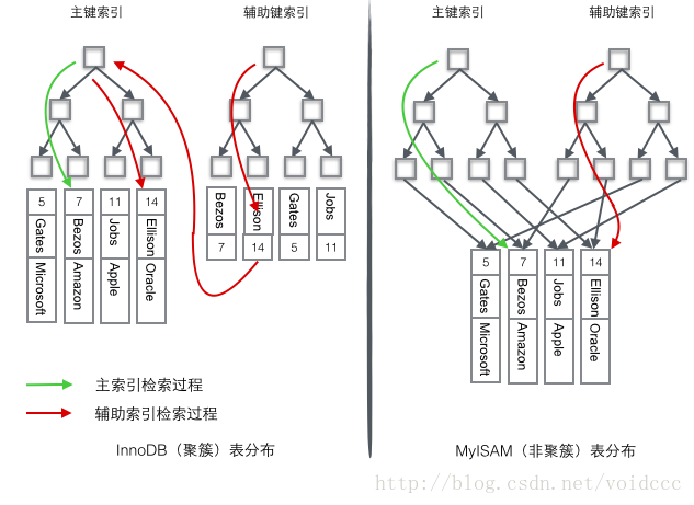
InnoDB使用的是聚簇索引,将主键组织到一棵B+树中,而行数据就储存在叶子节点上,若使用"where id = 14"这样的条件查找主键,则按照B+树的检索算法即可查找到对应的叶节点,之后获得行数据。若对Name列进行条件搜索,则需要两个步骤:第一步在辅助索引B+树中检索Name,到达其叶子节点获取对应的主键。第二步使用主键在主索引B+树种再执行一次B+树检索操作,最终到达叶子节点即可获取整行数据。
MyISM使用的是非聚簇索引,非聚簇索引的两棵B+树看上去没什么不同,节点的结构完全一致只是存储的内容不同而已,主键索引B+树的节点存储了主键,辅助键索引B+树存储了辅助键。表数据存储在独立的地方,这两颗B+树的叶子节点都使用一个地址指向真正的表数据,对于表数据来说,这两个键没有任何差别。由于索引树是独立的,通过辅助键检索无需访问主键的索引树。
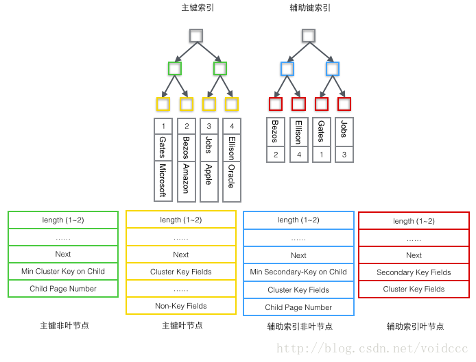
为了更形象说明这两种索引的区别,我们假想一个表如下图存储了4行数据。其中Id作为主索引,Name作为辅助索引。图示清晰的显示了聚簇索引和非聚簇索引的差异。

我们重点关注聚簇索引,看上去聚簇索引的效率明显要低于非聚簇索引,因为每次使用辅助索引检索都要经过两次B+树查找,这不是多此一举吗?聚簇索引的优势在哪?
1 由于行数据和叶子节点存储在一起,这样主键和行数据是一起被载入内存的,找到叶子节点就可以立刻将行数据返回了,如果按照主键Id来组织数据,获得数据更快。
2 辅助索引使用主键作为"指针" 而不是使用地址值作为指针的好处是,减少了当出现行移动或者数据页分裂时辅助索引的维护工作,使用主键值当作指针会让辅助索引占用更多的空间,换来的好处是InnoDB在移动行时无须更新辅助索引中的这个"指针"。也就是说行的位置(实现中通过16K的Page来定位,后面会涉及)会随着数据库里数据的修改而发生变化(前面的B+树节点分裂以及Page的分裂),使用聚簇索引就可以保证不管这个主键B+树的节点如何变化,辅助索引树都不受影响。
3 Page结构
如果说前面的内容偏向于解释原理,那后面就开始涉及具体实现了。
理解InnoDB的实现不得不提Page结构,Page是整个InnoDB存储的最基本构件,也是InnoDB磁盘管理的最小单位,与数据库相关的所有内容都存储在这种Page结构里。Page分为几种类型,常见的页类型有数据页(B-tree Node)Undo页(Undo Log Page)系统页(System Page) 事务数据页(Transaction System Page)等。单个Page的大小是16K(编译宏UNIV_PAGE_SIZE控制),每个Page使用一个32位的int值来唯一标识,这也正好对应InnoDB最大64TB的存储容量(16Kib * 2^32 = 64Tib)。一个Page的基本结构如下图所示:

每个Page都有通用的头和尾,但是中部的内容根据Page的类型不同而发生变化。Page的头部里有我们关心的一些数据,下图把Page的头部详细信息显示出来:
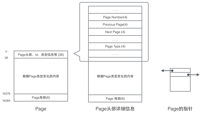
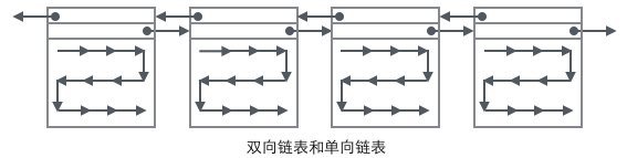
我们重点关注和数据组织结构相关的字段:Page的头部保存了两个指针,分别指向前一个Page和后一个Page,头部还有Page的类型信息和用来唯一标识Page的编号。根据这两个指针我们很容易想象出Page链接起来就是一个双向链表的结构。

再看看Page的主体内容,我们主要关注行数据和索引的存储,他们都位于Page的User Records部分,User Records占据Page的大部分空间,User Records由一条一条的Record组成,每条记录代表索引树上的一个节点(非叶子节点和叶子节点)。在一个Page内部,单链表的头尾由固定内容的两条记录来表示,字符串形式的"Infimum"代表开头,"Supremum"代表结尾。这两个用来代表开头结尾的Record存储在System Records的段里,这个System Records和User Records是两个平行的段。InnoDB存在4种不同的Record,它们分别是1主键索引树非叶节点 2主键索引树叶子节点 3辅助键索引树非叶节点 4辅助键索引树叶子节点。这4种节点的Record格式有一些差异,但是它们都存储着Next指针指向下一个Record。后续我们会详细介绍这4种节点,现在只需要把Record当成一个存储了数据同时含有Next指针的单链表节点即可。
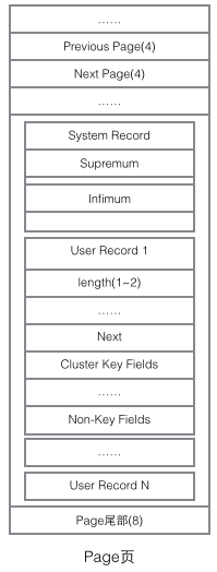
User Record在Page内以单链表的形式存在,最初数据是按照插入的先后顺序排列的,但是随着新数据的插入和旧数据的删除,数据物理顺序会变得混乱,但他们依然保持着逻辑上的先后顺序。

把User Record的组织形式和若干Page组合起来,就看到了稍微完整的形式。
现在看下如何定位一个Record:
1 通过根节点开始遍历一个索引的B+树,通过各层非叶子节点最终到达一个Page,这个Page里存放的都是叶子节点。
2 在Page内从"Infimum"节点开始遍历单链表(这种遍历往往会被优化),如果找到该键则成功返回。如果记录到达了"supremum",说明当前Page里没有合适的键,这时要借助Page的Next Page指针,跳转到下一个Page继续从"Infimum"开始逐个查找。

详细看下不同类型的Record里到底存储了什么数据,根据B+树节点的不同,User Record可以被分成四种格式,下图种按照颜色予以区分。
1 主索引树非叶节点(绿色)
1 子节点存储的主键里最小的值(Min Cluster Key on Child),这是B+树必须的,作用是在一个Page里定位到具体的记录的位置。
2 最小的值所在的Page的编号(Child Page Number),作用是定位Record。
2 主索引树叶子节点(黄色)
1 主键(Cluster Key Fields),B+树必须的,也是数据行的一部分
2 除去主键以外的所有列(Non-Key Fields),这是数据行的除去主键的其他所有列的集合。
这里的1和2两部分加起来就是一个完整的数据行。
3 辅助索引树非叶节点非(蓝色)
1 子节点里存储的辅助键值里的最小的值(Min Secondary-Key on Child),这是B+树必须的,作用是在一个Page里定位到具体的记录的位置。
2 主键值(Cluster Key Fields),非叶子节点为什么要存储主键呢?因为辅助索引是可以不唯一的,但是B+树要求键的值必须唯一,所以这里把辅助键的值和主键的值合并起来作为在B+树中的真正键值,保证了唯一性。但是这也导致在辅助索引B+树中非叶节点反而比叶子节点多了4个字节。(即下图中蓝色节点反而比红色多了4字节)
3 最小的值所在的Page的编号(Child Page Number),作用是定位Record。
4 辅助索引树叶子节点(红色)
1 辅助索引键值(Secondary Key Fields),这是B+树必须的。
2 主键值(Cluster Key Fields),用来在主索引树里再做一次B+树检索来找到整条记录。
下面是本篇最重要的部分了,结合B+树的结构和前面介绍的4种Record的内容,我们终于可以画出一幅全景图。由于辅助索引的B+树与主键索引有相似的结构,这里只画出了主键索引树的结构图,只包含了"主键非叶节点"和"主键叶子节点"两种节点,也就是上图的的绿色和黄色的部分。
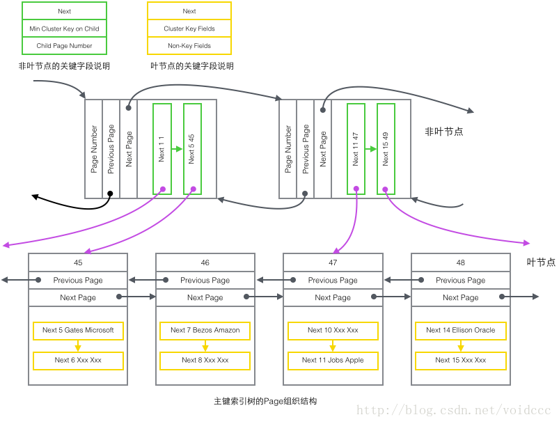
把上图还原成下面这个更简洁的树形示意图,这就是B+树的一部分。注意Page和B+树节点之间并没有一一对应的关系,Page只是作为一个Record的保存容器,它存在的目的是便于对磁盘空间进行批量管理,上图中的编号为47的Page在树形结构上就被拆分成了两个独立节点。

至此本篇就算结束了,本篇只是对InnoDB索引相关的数据结构和实现进行了一些梳理总结,并未涉及到Mysql的实战经验。这主要是基于几点原因:
1 原理是基石,只有充分了解InnoDB索引的工作方式,我们才有能力高效的使用好它。
2 原理性知识特别适合使用图示,我个人非常喜欢这种表达方式。
3 关于InnoDB优化,在《高性能Mysql》里有更加全面的介绍,对优化Mysql感兴趣的同学完全可以自己获取相关知识,我自己的积累还未达到能分享这些内容的地步。
另:对InnoDB实现有更多兴趣的同学可以看看Jeremy Cole的博客(参考文献三篇文章的来源),这位老兄曾先后在Mysql,Yahoo,Twitter,Google从事数据库相关工作,他的文章非常棒!
参考文献:
[1] Jeremy Cole The physical structure of InnoDB index pages
[2] Jeremy Cole B+Tree index structures in InnoDB
[3] Jeremy Cole The physical structure of records in InnoDB
[4] 姜承尧 MySQL技术内幕-InnoDB存储引擎 第二版
[5] Schwartz,B / Zaitsev,P / Tkach 高性能Mysql 第三版
[6] B-tree wiki
————————————————
https://blog.csdn.net/voidccc/article/details/40077329
MySQL :: MySQL 8.0 Reference Manual :: 13.1.20.9 Secondary Indexes and Generated Columns https://dev.mysql.com/doc/refman/8.0/en/create-table-secondary-indexes.html
13.1.20.9 Secondary Indexes and Generated Columns
InnoDB supports secondary indexes on virtual generated columns. Other index types are not supported. A secondary index defined on a virtual column is sometimes referred to as a “virtual index”.
A secondary index may be created on one or more virtual columns or on a combination of virtual columns and regular columns or stored generated columns. Secondary indexes that include virtual columns may be defined as UNIQUE.
When a secondary index is created on a virtual generated column, generated column values are materialized in the records of the index. If the index is a covering index (one that includes all the columns retrieved by a query), generated column values are retrieved from materialized values in the index structure instead of computed “on the fly”.
There are additional write costs to consider when using a secondary index on a virtual column due to computation performed when materializing virtual column values in secondary index records during INSERT and UPDATE operations. Even with additional write costs, secondary indexes on virtual columns may be preferable to generated stored columns, which are materialized in the clustered index, resulting in larger tables that require more disk space and memory. If a secondary index is not defined on a virtual column, there are additional costs for reads, as virtual column values must be computed each time the column's row is examined.
Values of an indexed virtual column are MVCC-logged to avoid unnecessary recomputation of generated column values during rollback or during a purge operation. The data length of logged values is limited by the index key limit of 767 bytes for COMPACT and REDUNDANT row formats, and 3072 bytes for DYNAMIC and COMPRESSED row formats.
Adding or dropping a secondary index on a virtual column is an in-place operation.
As noted elsewhere, JSON columns cannot be indexed directly. To create an index that references such a column indirectly, you can define a generated column that extracts the information that should be indexed, then create an index on the generated column, as shown in this example:
mysql> CREATE TABLE jemp (
    ->     c JSON,
    ->     g INT GENERATED ALWAYS AS (c->"$.id"),
    ->     INDEX i (g)
    -> );
Query OK, 0 rows affected (0.28 sec)

mysql> INSERT INTO jemp (c) VALUES
     >   ('{"id": "1", "name": "Fred"}'), ('{"id": "2", "name": "Wilma"}'),
     >   ('{"id": "3", "name": "Barney"}'), ('{"id": "4", "name": "Betty"}');
Query OK, 4 rows affected (0.04 sec)
Records: 4  Duplicates: 0  Warnings: 0

mysql> SELECT c->>"$.name" AS name
     >     FROM jemp WHERE g > 2;
+--------+
| name   |
+--------+
| Barney |
| Betty  |
+--------+
2 rows in set (0.00 sec)

mysql> EXPLAIN SELECT c->>"$.name" AS name
     >    FROM jemp WHERE g > 2\G
*************************** 1. row ***************************
           id: 1
  select_type: SIMPLE
        table: jemp
   partitions: NULL
         type: range
possible_keys: i
          key: i
      key_len: 5
          ref: NULL
         rows: 2
     filtered: 100.00
        Extra: Using where
1 row in set, 1 warning (0.00 sec)

mysql> SHOW WARNINGS\G
*************************** 1. row *********************