


插入排序 堆排序 归并排序 递归与非递归 希尔排序 选择排序 堆排序 比较交换 原地排序 非原地 稳定排序 非稳定 计数排序 基数排序 桶排序
http://www.cse.chalmers.se/edu/year/2018/course/DAT037/slides/3.pdf
Bucket Sort Algorithm - LearnersBucket https://learnersbucket.com/tutorials/algorithms/bucket-sort-algorithm/
Bucket Sort Data Structure and Algorithm with easy Example | lectureloops https://lectureloops.com/bucket-sort/
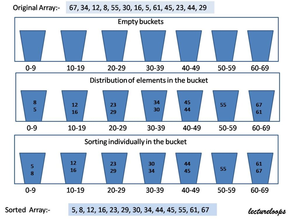
Consider an example,
67, 34, 12, 8, 55, 30, 16, 5, 61, 45, 23, 44, 29
Now we have to decide how many buckets we have to make? Well, you can have any criteria. One may be like, calculate the range of your values. The range is (maximum value – minimum value). The minimum element is 5. The maximum element is 67. The range is 67-5= 62. Then take the square root of range. If it is not an integer, then take floor value. The square root of 62:
floor(sqrt(62))=7. Therefore we can take 7 buckets of equal range. The buckets are numbered as 0 to 6.
- 0-9
- 10-19
- 20-29
- 30-39
- 40-49
- 50-59
- 60-69
Now you have to distribute elements in these buckets according to the range of buckets. For distributing elements you can have any hash function. Suppose in this particular example, we can divide elements by 10. Like 67/10 = 6. So 67 will go in the 6th bucket. (We are starting from 0). We can use it with floating-point values also. Then we can multiply with 10 instead of dividing. For example, if values are 0.47 or 0.23. Then perform floor(value*10). Then you will get 4 and 2. This 4 and 2 is the bucket number in that case.
We can implement these buckets with a linked list. Then we need to decide Which sorting algorithm to use to sort these buckets? We know that Insertion sort performs better if elements are almost sorted. Therefore we generally use insertion sort. But you can use other sorting techniques also.
func bucketSort(input []int) []int {
	// 非负的整数
	min, max := 0, 0
	for _, v := range input {
		if min > v {
			min = v
		}
		if max < v {
			max = v
		}
	}
	nearSquareRoot := func(a int) int {
		if a <= 4 {
			return 2
		}
		half := a / 2
		x := 0
		for i := 0; i < half; i++ {
			y := i * i
			if y > a {
				return x
			}
			x = i
		}
		return x
	}
	bucketNum := nearSquareRoot(max-min) + 1
	bucket := make([][]int, bucketNum)
	for _, v := range input {
		u := v - min
		u = nearSquareRoot(u)
		bucket[u] = append(bucket[u], v)
	}
	var insertSort func(input []int) []int
	insertSort = func(input []int) []int {
		n := len(input)
		for i := 1; i < n; i++ {
			valueToInsert := input[i]
			j := i - 1
			for j >= 0 && input[j] > valueToInsert {
				input[j+1] = input[j]
				j--
			}
			input[j+1] = valueToInsert
		}
		return input
	}
	ans := []int{}
	for _, v := range bucket {
		v = insertSort(v)
		ans = append(ans, v...)
	}
	return ans
}
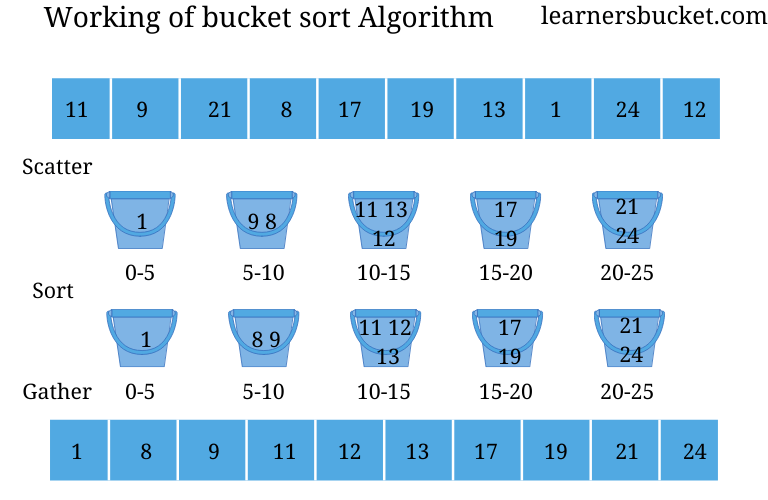
Like its cousin Radix sort, bucket sort also uses the element as the index for grouping, thus it cannot work on other data structure, we can sort the array of characters or string by using a hashing method where we convert the value to the numeric index.
//Add the elements in a same range in bucket
- 中文名
- 桶排序
- 要 求
- 数据的长度必须完全一样
- 公 式
- Data=rand()/10000+10000
- 数据结构设计
- 链表可以采用很多种方式实现
- 性 质
- 平均情况下桶排序以线性时间运行
- 原 理
- 桶排序利用函数的映射关系
- 领 域
- 计算机算法
代价
海量数据
典型
注意:
计数排序是可以为稳定排序的,虽然稳定排序、不稳定排序的结果一样;
在基数排序中使用计数排序,要求为稳定的计数排序。
func radixS(input []int) []int {
	n := len(input)
	if n < 2 {
		return input
	}
	// 非负的整数
	max := input[0]
	for _, v := range input {
		if v > max {
			max = v
		}
	}
	var countingSort func(exp int)
	countingSort = func(exp int) {
		counter := make([]int, 10)
		for i := 0; i < n; i++ {
			v := input[i]
			u := (v / exp) % 10
			counter[u]++
		}
		for i := 1; i < 10; i++ {
			counter[i] += counter[i-1]
		}
		ans := make([]int, n)
		for i := n - 1; i >= 0; i-- {
			// 注意:这一行,很关键,要求为稳定排序。
			// 不稳定排序: for i := 0; i < n; i-- {
			v := input[i]
			u := (v / exp) % 10
			index := counter[u] - 1
			ans[index] = v
			counter[u]--
		}
		input = ans
	}
	for exp := 1; max/exp > 0; exp *= 10 {
		countingSort(exp)
	}
	return input
}
基数排序
基于计数排序 计数排序为计数排序的子程序 subroutine
170, 45, 75, 90, 802, 24, 2, 66
1
170, 90,802,2, 24, 45, 75,66
10
802,2, 24, 45, 66,75,170, 90
100
2, 24, 45, 66,75, 90,170, 802
依次从个位、十位、百位、、、、、、保证顺序,最终保证了完成了排序。
基数排序解决的问题:
What if the elements are in the range from 1 to n2?
降低计数排序的元素个数
The lower bound for Comparison based sorting algorithm (Merge Sort, Heap Sort, Quick-Sort .. etc) is Ω(nLogn), i.e., they cannot do better than nLogn. Counting sort is a linear time sorting algorithm that sort in O(n+k) time when elements are in the range from 1 to k.
What if the elements are in the range from 1 to n2?
We can’t use counting sort because counting sort will take O(n2) which is worse than comparison-based sorting algorithms. Can we sort such an array in linear time?
Radix Sort is the answer. The idea of Radix Sort is to do digit by digit sort starting from least significant digit to most significant digit. Radix sort uses counting sort as a subroutine to sort.
The Radix Sort Algorithm
Do the following for each digit i where i varies from the least significant digit to the most significant digit. Here we will be sorting the input array using counting sort (or any stable sort) according to the i’th digit.
应用场景、优势
What is the running time of Radix Sort?
Let there be d digits in input integers. Radix Sort takes O(d*(n+b)) time where b is the base for representing numbers, for example, for the decimal system, b is 10. What is the value of d? If k is the maximum possible value, then d would be O(logb(k)). So overall time complexity is O((n+b) * logb(k)). Which looks more than the time complexity of comparison-based sorting algorithms for a large k. Let us first limit k. Let k <= nc where c is a constant. In that case, the complexity becomes O(nLogb(n)). But it still doesn’t beat comparison-based sorting algorithms.
What if we make the value of b larger?. What should be the value of b to make the time complexity linear? If we set b as n, we get the time complexity as O(n). In other words, we can sort an array of integers with a range from 1 to nc if the numbers are represented in base n (or every digit takes log2(n) bits).
Applications of Radix Sort:
- In a typical computer, which is a sequential random-access machine, where the records are keyed by multiple fields radix sort is used. For eg., you want to sort on three keys month, day and year. You could compare two records on year, then on a tie on month and finally on the date. Alternatively, sorting the data three times using Radix sort first on the date, then on month, and finally on year could be used.
- It was used in card sorting machines that had 80 columns, and in each column, the machine could punch a hole only in 12 places. The sorter was then programmed to sort the cards, depending upon which place the card had been punched. This was then used by the operator to collect the cards which had the 1st row punched, followed by the 2nd row, and so on.
Is Radix Sort preferable to Comparison based sorting algorithms like Quick-Sort?
If we have log2n bits for every digit, the running time of Radix appears to be better than Quick Sort for a wide range of input numbers. The constant factors hidden in asymptotic notation are higher for Radix Sort and Quick-Sort uses hardware caches more effectively. Also, Radix sort uses counting sort as a subroutine and counting sort takes extra space to sort numbers.
Key points about Radix Sort:
Some key points about radix sort are given here
- It makes assumptions about the data like the data must be between a range of elements.
- Input array must have the elements with the same radix and width.
- Radix sort works on sorting based on individual digit or letter position.
- We must start sorting from the rightmost position and use a stable algorithm at each position.
- Radix sort is not an in-place algorithm as it uses a temporary count array.
Radix Sort - GeeksforGeeks https://www.geeksforgeeks.org/radix-sort/
1.8 计数排序 | 菜鸟教程 https://www.runoob.com/w3cnote/counting-sort.html
func countingSort(input []int) []int {
	length := len(input)
	if length <= 1 {
		return input
	}
	// 非负的整数
	maxVal := input[0]
	for _, v := range input {
		if v > maxVal {
			maxVal = v
		}
	}
	bucketLen := maxVal + 1
	bucket := make([]int, bucketLen)
	sortedIndex := 0
	for i := 0; i < length; i++ {
		bucket[input[i]] += 1
	}
	for j := 0; j < bucketLen; j++ {
		for bucket[j] > 0 {
			input[sortedIndex] = j
			sortedIndex += 1
			bucket[j] -= 1
		}
	}
	return input
}
Counting Sort | Brilliant Math & Science Wiki https://brilliant.org/wiki/counting-sort/
func countingSort(input []int) []int {
	max := 0
	for _, v := range input {
		if v > max {
			max = v
		}
	}
	counter := make([]int, max+1)
	for _, v := range input {
		counter[v]++
	}
	ans := make([]int, 0)
	for v, n := range counter {
		for i := 0; i < n; i++ {
			ans = append(ans, v)
		}
	}
	return ans
}
func countingSort(input []int) []int {
	n := len(input)
	if n <= 1 {
		return input
	}
	// 非负的整数
	max := input[0]
	for _, v := range input {
		if v > max {
			max = v
		}
	}
	_len := max + 1
	counter := make([]int, _len)
	for _, v := range input {
		counter[v]++
	}
	for i := 1; i < _len; i++ {
		counter[i] += counter[i-1]
		// 排序后的,累计出现的频次,即排序后的名次
	}
	ans := make([]int, n)
	//	for i := 0; i < n; i++ { // 不稳定排序
	for i := n - 1; i >= 0; i-- { // 稳定排序
		v := input[i]
		index := counter[v] - 1
		ans[index] = v
		counter[v]--
	}
	return ans
}
考虑有负整数的情况
func countingSort(input []int) []int {
	n := len(input)
	if n <= 1 {
		return input
	}
	max, min := input[0], input[0]
	for _, v := range input {
		if v > max {
			max = v
		}
		if v < min {
			min = v
		}
	}
	negative := min < 0
	if negative {
		max = input[0]
		for i := 0; i < n; i++ {
			v := input[i] - min
			if v > max {
				max = v
			}
			input[i] = v
		}
	}
	counter := make([]int, max+1)
	for _, v := range input {
		counter[v]++
	}
	ans := make([]int, 0)
	for v, n := range counter {
		u := v
		if negative {
			u += min
		}
		for i := 0; i < n; i++ {
			ans = append(ans, u)
		}
	}
	return ans
}
Counting sort is an efficient algorithm for sorting an array of elements that each have a nonnegative integer key, for example, an array, sometimes called a list, of positive integers could have keys that are just the value of the integer as the key, or a list of words could have keys assigned to them by some scheme mapping the alphabet to integers (to sort in alphabetical order, for instance). Unlike other sorting algorithms, such as mergesort, counting sort is an integer sorting algorithm, not a comparison based algorithm. While any comparison based sorting algorithm requires \Omega(n \lg n)Ω(nlgn) comparisons, counting sort has a running time of \Theta(n)Θ(n) when the length of the input list is not much smaller than the largest key value, kk, in the list. Counting sort can be used as a subroutine for other, more powerful, sorting algorithms such as radix sort.
计数排序算法不是基于比较交换的算法
子程序 支持多线程
空间换时间
Sorting
An algorithm that maps the following input/output pair is called a sorting algorithm:
Input: An array, AA, of size nn of orderable elements. A[0,1,...,n-1]A[0,1,...,n−1]
Output: A sorted permutation of AA, called BB, such that B[0] \leq B[1] \leq ... \leq B[n-1].B[0]≤B[1]≤...≤B[n−1].
Here is what it means for an array to be sorted.
An array AA is sorted if and only if for all i<ji<j, A[i] \leq A[j].\ _\squareA[i]≤A[j]. □
By convention, empty arrays and singleton arrays (arrays consisting of only one element) are always sorted. This is a key point for the base case of many sorting algorithms.
Complexity of Counting Sort
Counting sort has a O(k+n)O(k+n) running time.
The first loop goes through AA, which has nn elements. This step has a O(n)O(n) running time. The second loop iterates over kk, so this step has a running time of O(k)O(k). The third loop iterates through AA, so again, this has a running time of O(n)O(n). Therefore, the counting sort algorithm has a running time of O(k+n)O(k+n).
Counting sort is efficient if the range of input data, kk, is not significantly greater than the number of objects to be sorted, nn.
Counting sort is a stable sort with a space complexity of O(k + n)O(k+n).
func heapSort(input []int) []int {
	var heapfiy func(limit, i int)
	heapfiy = func(limit, i int) {
		largest, left, right := i, 2*i+1, 2*i+2
		if left < limit && input[largest] < input[left] {
			largest = left
		}
		if right < limit && input[largest] < input[right] {
			largest = right
		}
		if largest != i {
			input[i] ^= input[largest]
			input[largest] ^= input[i]
			input[i] ^= input[largest]
			heapfiy(limit, largest)
		}
	}
	n := len(input)
	h := n / 2
	// 8->4->3=6,7
	// 7->3->2=5,6
	// 保证父节点值最大:将大的上移到的父节点
	// 上移
	for i := h; i >= 0; i-- {
		heapfiy(n, i)
	}
	for i := n - 1; i > 0; i-- {
		// 将最大的元素移动的最末一个节点,完成数组的元素升序排列
		// 下移
		input[0] ^= input[i]
		input[i] ^= input[0]
		input[0] ^= input[i]
		heapfiy(i, 0)
	}
	return input
}
[1 2 3]
[3 2 1]
=== RUN Test_heapSort/g-3-2
[3 2 1]
[3 2 1]
=== RUN Test_heapSort/g-3-3
[2 1 3]
[3 1 2]
=== RUN Test_heapSort/g-3-4
[1 3 2]
[3 1 2]
=== RUN Test_heapSort/g-3-5
[3 1 2]
[3 1 2]
=== RUN Test_heapSort/g-3-6
[2 3 1]
[3 2 1]
=== RUN Test_heapSort/g-2-1
[1 2]
[2 1]
=== RUN Test_heapSort/g-2-2
[2 1]
[2 1]
=== RUN Test_heapSort/x-0
[]
[]
=== RUN Test_heapSort/x-1
[1]
[1]
=== RUN Test_heapSort/1
[3 2 4 1]
[4 2 3 1]
=== RUN Test_heapSort/2
[6 202 100 301 38 8 1]
[301 202 100 6 38 8 1]
=== RUN Test_heapSort/3
[6 1 202 100 301 38 8 1]
[301 100 202 6 1 38 8 1]
=== RUN Test_heapSort/4
[10 1 3 56 13 59]
[59 56 10 1 13 3]
堆的存储:可以通过数组记录,保证(i,2i+1,2i+2)或者(n/2-1,n-1,n)的大小关系,及i或者n/2-1为最值。
小顶锥建立过程:
0、堆化:实现一个节点的父节点比子节点大、子节点比子节点的子节点大,递归实现;
1、遍历节点[0,n/2-1],堆化,实现任一个节点的父节点比子节点大;
2、遍历节点(0,n-1],交换根节点和当前节点的值,然后堆化。
小顶锥 > largest
大顶锥 < smallest
HeapSort - GeeksforGeeks https://www.geeksforgeeks.org/heap-sort/
Heap sort is a comparison-based sorting technique based on Binary Heap data structure. It is similar to selection sort where we first find the minimum element and place the minimum element at the beginning. We repeat the same process for the remaining elements.
What is Binary Heap?
Let us first define a Complete Binary Tree. A complete binary tree is a binary tree in which every level, except possibly the last, is completely filled, and all nodes are as far left as possible (Source Wikipedia)
A Binary Heap is a Complete Binary Tree where items are stored in a special order such that the value in a parent node is greater(or smaller) than the values in its two children nodes. The former is called max heap and the latter is called min-heap. The heap can be represented by a binary tree or array.
Why array based representation for Binary Heap?
Since a Binary Heap is a Complete Binary Tree, it can be easily represented as an array and the array-based representation is space-efficient. If the parent node is stored at index I, the left child can be calculated by 2 * I + 1 and the right child by 2 * I + 2 (assuming the indexing starts at 0).
How to “heapify” a tree?
The process of reshaping a binary tree into a Heap data structure is known as ‘heapify’. A binary tree is a tree data structure that has two child nodes at max. If a node’s children nodes are ‘heapified’, then only ‘heapify’ process can be applied over that node. A heap should always be a complete binary tree.
Starting from a complete binary tree, we can modify it to become a Max-Heap by running a function called ‘heapify’ on all the non-leaf elements of the heap. i.e. ‘heapify’ uses recursion.
Algorithm for “heapify”:
heapify(array)
Root = array[0]Largest = largest( array[0] , array [2 * 0 + 1]. array[2 * 0 + 2])
if(Root != Largest)
Swap(Root, Largest)
Example of “heapify”:
30(0)
/ \
70(1) 50(2)Child (70(1)) is greater than the parent (30(0))
Swap Child (70(1)) with the parent (30(0))
70(0)
/ \
30(1) 50(2)
Heap Sort Algorithm for sorting in increasing order:
- Build a max heap from the input data.
- At this point, the largest item is stored at the root of the heap. Replace it with the last item of the heap followed by reducing the size of heap by 1. Finally, heapify the root of the tree.
- Repeat step 2 while the size of the heap is greater than 1.
How to build the heap?
Heapify procedure can be applied to a node only if its children nodes are heapified. So the heapification must be performed in the bottom-up order.
Lets understand with the help of an example:
How heap sort works?
- To understand heap sort more clearly, let’s take an unsorted array and try to sort it using heap sort.
- After that, the task is to construct a tree from that unsorted array and try to convert it into max heap.
- To transform a heap into a max-heap, the parent node should always be greater than or equal to the child nodes
- Here, in this example, as the parent node 4 is smaller than the child node 10, thus, swap them to build a max-heap.
- Now, as seen, 4 as a parent is smaller than the child 5, thus swap both of these again and the resulted heap and array should be like this:
- Next, simply delete the root element (10) from the max heap. In order to delete this node, try to swap it with the last node, i.e. (1). After removing the root element, again heapify it to convert it into max heap.
- Resulted heap and array should look like this:
- After repeating the above steps, at last swap first and last node and delete the last node from heap, and thus the resulted array seems to be the sorted one as shown in figure:
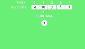
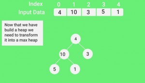
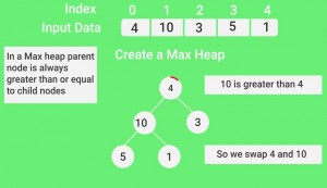
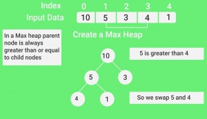
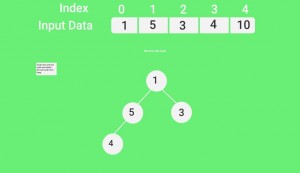
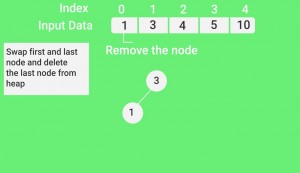
Illustration:
Input data: {4, 10, 3, 5, 1}
4(0)
/ \
10(1) 3(2)
/ \
5(3) 1(4)The numbers in bracket represent the indices in the array representation of data.
Applying heapify procedure to index 1:
4(0)
/ \
10(1) 3(2)
/ \
5(3) 1(4)Applying heapify procedure to index 0:
10(0)
/ \
5(1) 3(2)
/ \
4(3) 1(4)The heapify procedure calls itself recursively to build heap in top down manner.
Heap sort is a comparison-based sorting technique based on Binary Heap data structure. It is similar to selection sort where we first find the minimum element and place the minimum element at the beginning. We repeat the same process for the remaining elements.
堆排序基于比较、类似选择排序
Selection Sort (With Code in Python/C++/Java/C) https://www.programiz.com/dsa/selection-sort
selectionSort(array, size)
  repeat (size - 1) times
  set the first unsorted element as the minimum
  for each of the unsorted elements
    if element < currentMinimum
      set element as new minimum
  swap minimum with first unsorted position
end selectionSort
Selection Sort In Java - onlinetutorialspoint https://www.onlinetutorialspoint.com/java/selection-sort-in-java.html
Selection Sort https://www.tutorialspoint.com/Selection-Sort
Begin
   for i := 0 to size-2 do //find minimum from ith location to size
      iMin := i;
      for j:= i+1 to size – 1 do
         if array[j] < array[iMin] then
            iMin := j
      done
      swap array[i] with array[iMin].
   done
End
In the selection sort technique, the list is divided into two parts. In one part all elements are sorted and in another part the items are unsorted. At first, we take the maximum or minimum data from the array. After getting the data (say minimum) we place it at the beginning of the list by replacing the data of first place with the minimum data. After performing the array is getting smaller. Thus this sorting technique is done.
The complexity of Selection Sort Technique
- Time Complexity: O(n^2)
- Space Complexity: O(1)
func selectionSort(input []int) []int {
	n := len(input)
	for left := 0; left < n; left++ {
		min := left
		for right := left + 1; right < n; right++ {
			if input[min] > input[right] {
				min = right
			}
		}
		if min != left {
			input[left] ^= input[min]
			input[min] ^= input[left]
			input[left] ^= input[min]
		}
	}
	return input
}
func shellSort(input []int) []int {
	var interval int
	n := len(input)
	for interval < n {
		interval = interval*3 + 1
	}
	for interval > 0 {
		for right := interval; right < n; right++ {
			valueToInsert := input[right]
			var swaped bool
			left := right
			for left-interval >= 0 && input[left-interval] > valueToInsert {
				input[left] = input[left-interval]
				swaped = true
				left -= interval
			}
			if swaped {
				input[left] = valueToInsert
			}
		}
		interval = (interval - 1) / 3
	}
	return input
}
GitHub - heray1990/AlgorithmVisualization: Visually shows sorting algorithms with Python. https://github.com/heray1990/AlgorithmVisualization
Shell sort | R Data Structures and Algorithms https://subscription.packtpub.com/book/application-development/9781786465153/5/ch05lvl1sec32/shell-sort
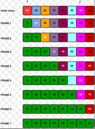
Shell sort (also called diminishing increment sort) is a non-intuitive (real-life) and a non-adjacent element comparison (and swap) type of sorting algorithm. It is a derivative of insertion sorting; however, it performs way better in worst-case scenarios. It is based on a methodology adopted by many other algorithms to be covered later: the entire vector (parent) is initially split into multiple subvectors (child), then sorting is performed on each subvector, and later all the subvectors are recombined into their parent vector.
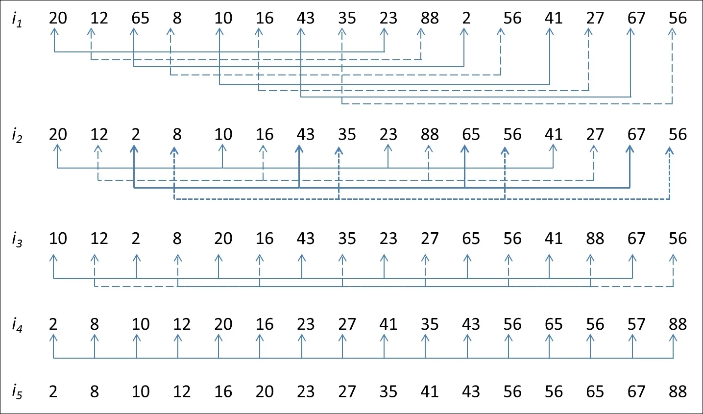
Shell sort, in general, splits each vector into virtual subvectors. These subvectors are disjointed such that each element in a subvector is a fixed number of positions apart. Each subvector is sorted using insertion sort. The process of selecting a subvector and sorting continues till the entire vector is sorted. Let us understand the process in detail using an example and illustration (Figure 5.5):
Shell Sort Algorithm in C, C++, Java with Examples | FACE Prep https://www.faceprep.in/c/shell-sort-algorithm-in-c/
Shell sort algorithm is very similar to that of the Insertion sort algorithm. In case of Insertion sort, we move elements one position ahead to insert an element at its correct position. Whereas here, Shell sort starts by sorting pairs of elements far apart from each other, then progressively reducing the gap between elements to be compared. Starting with far apart elements, it can move some out-of-place elements into the position faster than a simple nearest-neighbor exchange.
ShellSort - GeeksforGeeks https://www.geeksforgeeks.org/shellsort/
Data Structure and Algorithms - Shell Sort https://www.tutorialspoint.com/data_structures_algorithms/shell_sort_algorithm.htm
We see that it required only four swaps to sort the rest of the array.
Algorithm
Following is the algorithm for shell sort.
Step 1 − Initialize the value of h
Step 2 − Divide the list into smaller sub-list of equal interval h
Step 3 − Sort these sub-lists using insertion sort
Step 3 − Repeat until complete list is sorted
Pseudocode
Following is the pseudocode for shell sort.
procedure shellSort()
   A : array of items

   /* calculate interval*/
   while interval < A.length /3 do:
      interval = interval * 3 + 1
   end while

   while interval > 0 do:

      for outer = interval; outer < A.length; outer ++ do:

      /* select value to be inserted */
      valueToInsert = A[outer]
      inner = outer;

         /*shift element towards right*/
         while inner > interval -1 && A[inner - interval] >= valueToInsert do:
            A[inner] = A[inner - interval]
            inner = inner - interval
         end while

      /* insert the number at hole position */
      A[inner] = valueToInsert

      end for

   /* calculate interval*/
   interval = (interval -1) /3;

   end while

end procedure
ShellSort
Shell sort is mainly a variation of Insertion Sort. In insertion sort, we move elements only one position ahead. When an element has to be moved far ahead, many movements are involved. The idea of ShellSort is to allow the exchange of far items. In Shell sort, we make the array h-sorted for a large value of h. We keep reducing the value of h until it becomes 1. An array is said to be h-sorted if all sublists of every h’th element are sorted.
Algorithm:
Step 1 − Start
Step 2 − Initialize the value of gap size. Example: h
Step 3 − Divide the list into smaller sub-part. Each must have equal intervals to h
Step 4 − Sort these sub-lists using insertion sort
Step 5 – Repeat this step 2 until the list is sorted.
Step 6 – Print a sorted list.
Step 7 – Stop.
Pseudocode :
PROCEDURE SHELL_SORT(ARRAY, N)
WHILE GAP < LENGTH(ARRAY) /3 :
GAP = ( INTERVAL * 3 ) + 1
END WHILE LOOP
WHILE GAP > 0 :
FOR (OUTER = GAP; OUTER < LENGTH(ARRAY); OUTER++):
INSERTION_VALUE = ARRAY[OUTER]
INNER = OUTER;
WHILE INNER > GAP-1 AND ARRAY[INNER – GAP] >= INSERTION_VALUE:
ARRAY[INNER] = ARRAY[INNER – GAP]
INNER = INNER – GAP
END WHILE LOOP
ARRAY[INNER] = INSERTION_VALUE
END FOR LOOP
GAP = (GAP -1) /3;
END WHILE LOOP
END SHELL_SORT
希尔排序是插入排序的变种
希尔排序基于插入排序
Shell sort is a highly efficient sorting algorithm and is based on insertion sort algorithm. This algorithm avoids large shifts as in case of insertion sort, if the smaller value is to the far right and has to be moved to the far left.
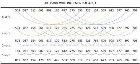
This algorithm uses insertion sort on a widely spread elements, first to sort them and then sorts the less widely spaced elements. This spacing is termed as interval. This interval is calculated based on Knuth's formula as −
Knuth's Formula
h = h * 3 + 1
where −
h is interval with initial value 1
This algorithm is quite efficient for medium-sized data sets as its average and worst-case complexity of this algorithm depends on the gap sequence the best known is Ο(n), where n is the number of items. And the worst case space complexity is O(n).
func insertSort(input []int) []int {
	n := len(input)
	for right := 1; right < n; right++ {
		valueToInsert := input[right]
		left := right - 1
		for left >= 0 && input[left] > valueToInsert {
			input[left+1] = input[left]
			left--
		}
		input[left+1] = valueToInsert
	}
	return input
}
Insertion Sort - GeeksforGeeks https://www.geeksforgeeks.org/insertion-sort/
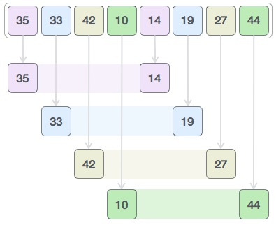
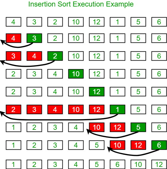
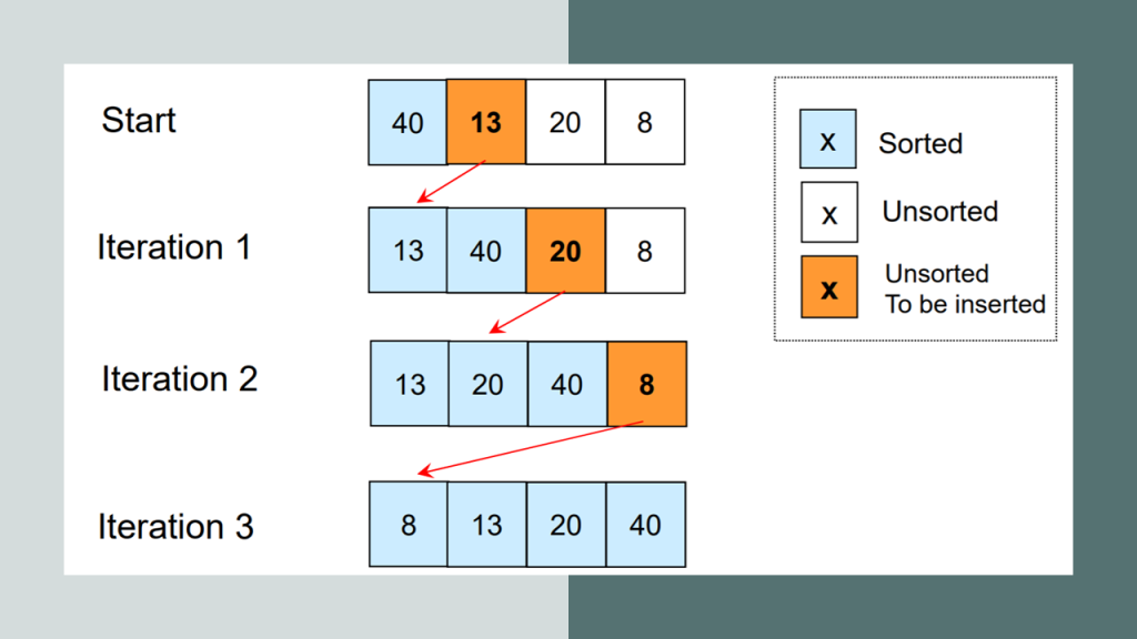
Insertion sort is a simple sorting algorithm that works similar to the way you sort playing cards in your hands. The array is virtually split into a sorted and an unsorted part. Values from the unsorted part are picked and placed at the correct position in the sorted part.
Characteristics of Insertion Sort:
- This algorithm is one of the simplest algorithm with simple implementation
- Basically, Insertion sort is efficient for small data values
- Insertion sort is adaptive in nature, i.e. it is appropriate for data sets which are already partially sorted.
插入排序:打扑克牌,调整手中牌的顺序。
Insertion Sort in C++ https://thecleverprogrammer.com/2020/11/15/insertion-sort-in-c/
Insertion Sort Algorithm
To sort an array of size N in ascending order:
- Iterate from arr[1] to arr[N] over the array.
- Compare the current element (key) to its predecessor.
- If the key element is smaller than its predecessor, compare it to the elements before. Move the greater elements one position up to make space for the swapped element.
5 6 11 12 13
Time Complexity: O(N^2)
Auxiliary Space: O(1)
What are the Boundary Cases of Insertion Sort algorithm?
Insertion sort takes maximum time to sort if elements are sorted in reverse order. And it takes minimum time (Order of n) when elements are already sorted.
What are the Algorithmic Paradigm of Insertion Sort algorithm?
Insertion Sort algorithm follows incremental approach.
Is Insertion Sort an in-place sorting algorithm?
Yes, insertion sort is an in-place sorting algorithm.
Is Insertion Sort a stable algorithm?
Yes, insertion sort is a stable sorting algorithm.
When is the Insertion Sort algorithm used?
Insertion sort is used when number of elements is small. It can also be useful when input array is almost sorted, only few elements are misplaced in complete big array.
What is Binary Insertion Sort?
We can use binary search to reduce the number of comparisons in normal insertion sort. Binary Insertion Sort uses binary search to find the proper location to insert the selected item at each iteration. In normal insertion, sorting takes O(i) (at ith iteration) in worst case. We can reduce it to O(logi) by using binary search. The algorithm, as a whole, still has a running worst case running time of O(n^2) because of the series of swaps required for each insertion. Refer this for implementation.
How to implement Insertion Sort for Linked List?
Below is simple insertion sort algorithm for linked list.
- Create an empty sorted (or result) list
- Traverse the given list, do following for every node.
- Insert current node in sorted way in sorted or result list.
- Change head of given linked list to head of sorted (or result) list.
QuickSort - GeeksforGeeks https://www.geeksforgeeks.org/quick-sort/
Like Merge Sort, QuickSort is a Divide and Conquer algorithm. It picks an element as pivot and partitions the given array around the picked pivot. There are many different versions of quickSort that pick pivot in different ways.
- Always pick first element as pivot.
- Always pick last element as pivot (implemented below)
- Pick a random element as pivot.
- Pick median as pivot.
The key process in quickSort is partition(). Target of partitions is, given an array and an element x of array as pivot, put x at its correct position in sorted array and put all smaller elements (smaller than x) before x, and put all greater elements (greater than x) after x. All this should be done in linear time.
merge sort
func mergeSort(input []int) []int {
	// DivideConquer
	var dv func(input []int) []int
	dv = func(input []int) []int {
		n := len(input)
		if n <= 1 {
			return input
		}
		mid := n / 2
		left, right := dv(input[0:mid]), dv(input[mid:])
		ret := []int{}
		i, j := 0, 0
		for i < len(left) && j < len(right) {
			if left[i] < right[j] {
				ret = append(ret, left[i])
				i++
			} else {
				ret = append(ret, right[j])
				j++
			}
		}
		if i < len(left) {
			ret = append(ret, left[i:]...)
		} else {
			ret = append(ret, right[j:]...)
		}
		return ret
	}
	return dv(input)
}
Merge Sort - GeeksforGeeks https://www.geeksforgeeks.org/merge-sort/
Like QuickSort, Merge Sort is a Divide and Conquer algorithm. It divides the input array into two halves, calls itself for the two halves, and then it merges the two sorted halves. The merge() function is used for merging two halves. The merge(arr, l, m, r) is a key process that assumes that arr[l..m] and arr[m+1..r] are sorted and merges the two sorted sub-arrays into one.
Pseudocode :
•    Declare left variable to 0 and right variable to n-1
•    Find mid by medium formula. mid = (left+right)/2
•    Call merge sort on (left,mid)
•    Call merge sort on (mid+1,rear)
•    Continue till left is less than right
•    Then call merge function to perform merge sort.
Algorithm:
step 1: start
step 2: declare array and left, right, mid variable
step 3: perform merge function.
        mergesort(array,left,right)
        mergesort (array, left, right)
        if left > right
        return
        mid= (left+right)/2
        mergesort(array, left, mid)
        mergesort(array, mid+1, right)
        merge(array, left, mid, right)
step 4: Stop
See the following C implementation for details.
Computer Science An Overview _J. Glenn Brookshear _11th Edition
procedure Sort (List)
N ← 2;
while (the value of N does not exceed the length of List)do
(
Select the Nth entry in List as the pivot entry;
Move the pivot entry to a temporary location leaving a hole in List;
while (there is a name above the hole and that name is greater than the pivot)
do (move the name above the hole down into the hole leaving a hole above the name)
Move the pivot entry into the hole in List;
N ← N + 1)
//pivot entry 主元项
https://baike.baidu.com/item/归并排序/1639015
https://baike.baidu.com/item/选择排序/9762418
https://baike.baidu.com/item/插入排序/7214992
https://baike.baidu.com/item/快速排序算法/369842
https://baike.baidu.com/item/冒泡排序/4602306
排序算法
平均时间复杂度
冒泡排序
O(n²)
选择排序
O(n²)
插入排序
O(n²)
希尔排序
O(n1.5)
快速排序
O(N*logN)
归并排序
O(N*logN)
堆排序
O(N*logN)
基数排序
O(d(n+r))
题目:下述几种排序方法中,要求内存最大的是()
A、快速排序
B、插入排序
C、选择排序
D、归并排序
'''
https://baike.baidu.com/item/归并排序/1639015
https://baike.baidu.com/item/选择排序/9762418
https://baike.baidu.com/item/插入排序/7214992
https://baike.baidu.com/item/快速排序算法/369842

https://baike.baidu.com/item/冒泡排序/4602306

'''
def bubbleSort(arr):
    size=len(arr)
    if size in (0,1):
        return arr
    while size>0:
        for i in range(1,size,1):
            if arr[i-1]>arr[i]:
                arr[i-1],arr[i]=arr[i],arr[i-1] # 冒泡,交换位置
        size-=1
    return arr

for i in range(1,3,1):
    print(i)

arrs=[[],[1],[1,2],[2,1],[3,2,1]]
for i in arrs:
    print(bubbleSort(i))
'''
n-1<=C<=n(n-1)/2
'''


def quickSort(arr):
    size = len(arr)
    if size >= 2:
        mid_index = size // 2
        mid = arr[mid_index]
        left, right = [], []
        for i in range(size):
            if i == mid_index:
                continue
            num = arr[i]
            if num >= mid:
                right.append(num)
            else:
                left.append(num)
        return quickSort(left) + [mid] + quickSort(right)
    else:
        return arr


print(quickSort(arr))

'''
理想的情况是,每次划分所选择的中间数恰好将当前序列几乎等分,经过log2n趟划分,便可得到长度为1的子表。这样,整个算法的时间复杂度为O(nlog2n)。 [4]
最坏的情况是,每次所选的中间数是当前序列中的最大或最小元素,这使得每次划分所得的子表中一个为空表,另一子表的长度为原表的长度-1。这样,长度为n的数据表的快速排序需要经过n趟划分,使得整个排序算法的时间复杂度为O(n2)。
'''


def selectSort(arr):
    '''
    TODO 优化
    '''
    ret = []
    ret_index = []
    size = len(arr)
    v = arr[0]
    for i in range(size):
        if i in ret_index:
            continue

        m = arr[i]
        if i + 1 < size:
            for j in range(i + 1, size):
                if j in ret_index:
                    continue
                n = arr[j]
                if n < m:
                    m = n
                    ret_index.append(j)
        else:
            ret_index.append(i)

        ret.append(m)
    return ret


print(selectSort(arr))


def merge(left, right):
    '''
归并操作,也叫归并算法,指的是将两个顺序序列合并成一个顺序序列的方法。
如 设有数列{6,202,100,301,38,8,1}
初始状态:6,202,100,301,38,8,1
第一次归并后:{6,202},{100,301},{8,38},{1},比较次数:3;
第二次归并后:{6,100,202,301},{1,8,38},比较次数:4;
第三次归并后:{1,6,8,38,100,202,301},比较次数:4;
总的比较次数为:3+4+4=11;
逆序数为14;
    '''
    l, r, ret = 0, 0, []
    size_left, size_right = len(left), len(right)
    while l < size_left and l < size_right:
        if left[l] <= right[r]:
            ret.append(left[l])
            l += 1
        else:
            ret.append(right[r])
            r += 1
    if l < size_left:
        ret += left[l:]
    if r < size_right:
        ret += right[r:]
    return ret


def mergeSort(arr):
    size = len(arr)
    if size <= 1:
        return arr
    mid = size // 2
    left = arr[:mid]
    right = arr[mid:]
    return merge(left, right)


print(mergeSort(arr))
使用C语言实现12种排序方法_C 语言_脚本之家 https://www.jb51.net/article/177098.htm

Sort List (归并排序链表) - 排序链表 - 力扣(LeetCode) https://leetcode-cn.com/problems/sort-list/solution/sort-list-gui-bing-pai-xu-lian-biao-by-jyd/


插入排序
InsertSort
l = [666,1, 45, 6, 4, 6, 7, 89, 56, 343, 3, 212, 31, 1, 44, 5, 1, 12, 34, 442]
# l =  [666, 89, 44]
print(l)
sentry = 0
for i in range(1, len(l), 1):
    if l[i] < l[i - 1]:
        sentry = l[i]
        l[i] = l[i - 1]
        j = i - 2
        while sentry < l[j] and j >= 0:
            l[j + 1] = l[j]
            j -= 1
        l[j + 1] = sentry

print(l)
希尔排序
def InsertSort(l):
    sentry = 0
    for i in range(1, len(l), 1):
        if l[i] < l[i - 1]:
            sentry = l[i]
            l[i] = l[i - 1]
            j = i - 2
            while sentry < l[j] and j >= 0:
                l[j + 1] = l[j]
                j -= 1
            l[j + 1] = sentry
    return l


def f(l, d):
    length = len(l)
    part = []
    new_l = l
    for i in range(0, length, 1):

        for j in range(i, length, d):
            part.append(l[j])
        # print("part-1",part)
        part = InsertSort(part)
        # print("part-2",part)

        for j in range(i, length, d):
            new_l[j] = part[0]
            part = part[1:]

    return new_l

l, dk = [666, 1, 45, 6, 4, 6, 7, 89, 56, 343, 3, 212, 31, 1, 44, 5, 1, 12, 34, 442], [7, 5, 3, 1]
print(l)
for i in dk:
    l = f(l, i)

print(l)

 浙公网安备 33010602011771号