PCA算法简介

PCA是一种能够通过提取数据主成分达到数据降维目的的无监督算法。

因为数据之间（如自然图像的像素值）间都是存在冗余的，通过PCA可以将维度为256降到一个较低的近似向量。

通过一个2D降到1D的例子来理解一下PCA的原理。假设有如下一堆二维数据，我们通过SVD奇异值变换可以找到，代表这堆数据的两个方向（特征向量的方向，为什么是特征向量，特征值呢？）

 

怎么进行SVD变换呢？我们先计算这堆数据的协方差矩阵如下：

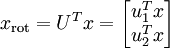
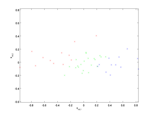
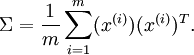数据变化的主方向就是sigma的主特征向量，次方向就是sigma的次特征向量。接下来我们计算旋转后的数据（也就是说把数据投影到以这两个特征方向为坐标轴的坐标平面内）

如图：

 

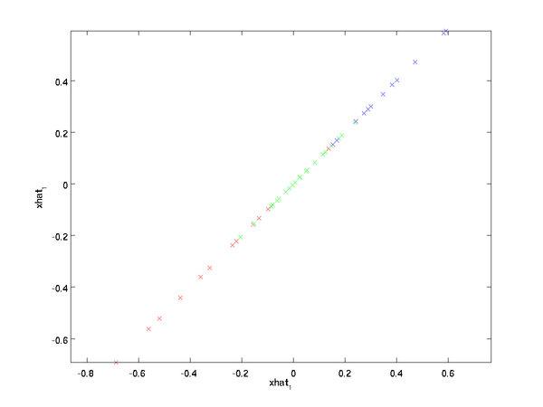
当我们只选取前面的k个主特征向量时，我们转换后就得到的是数据的主成分。PCA就是这样达到数据降维的。这里k=1,即选取主特征向量，得到数据的近似表示如下：、

 

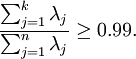
一般我们根据近似误差的要求来选取k。代表sigma协方差矩阵的特征值，一般地选择k保留百分之90的方差：

 

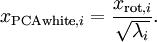
PCA经常和白化一起对图像进行预处理。PCA消除了输入特征间相关性。而白化之前要求的特征之间的低相关性要求正好就满足了。通过白化可以降低数据之间的冗余性。为了使得输入特征具有单位方差，我们利用作为缩放因子对进行缩放。得到：

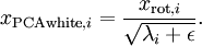
在实际中，我们往往给分母加入一个常量。

 

 

本文参照斯坦福UFLDL教程。http://deeplearning.stanford.edu/wiki/index.php/Exercise:PCA_in_2D

在matlab上实现这个例子代码如下：

close all
%%===============================================================
%%step0:Load data
% x is a 2*45 matrix,where the kth column x(:,k) corresponds to the
% kth data point.Here we provide the code to load natural image into x.
% You do not need to change the code below.

x = load('pcaData.txt','-ascii');
figure(1);
scatter(x(1,:),x(2,:));
title('Raw data');

%%=====================================================================
%step1a:Implement PCA to obtain U


u = zeros(size(x,1));%you need to campute this
[n m] = size(x);
x=x-repmat(mean(x,2),1,m);%预处理，均值为0
sigma = (1.0/m)*x*x'
[u s v]=svd(sigma);%svd函数其实计算的是矩阵的奇异值和奇异矩阵，但就半正定矩阵来说，它们对应于特征值和特征向量，
%那么矩阵U将包含sigma的特征向量（一个向量一列，从主向量开始排序），矩阵S对角线上的元素包含对应的特征值。矩阵V等于U的转制

hold on
plot([0 u(1,1)],[0 u(2,1)])%画第一条线
plot([0 u(1,2)],[0 u(2,2)])%画第二条线

%====================================================================
%step1b:compute xRot,the projection on to the eigenbasis
%Now,compute xRot by projecting the data on to the basis defined by
%U.Visualize the points by performing a scatter plot.

xRot = zeros(size(x));
xRot =u'*x;

%Visualize the covariance matrix.You should see a line across the diagonal
%against a blue backgroud.

figure(2);
scatter(xRot(1,:),xRot(2,:));
title('xRot');


%%=============================================================================
%step2;Reduce the number of dimensions from 2 to 1.
%Compute xRot again (this time project to 1 dimension)
%then,compute xHat by projecting the xRot back onto the original axes to
%see the effect of dimension reduction

k=1;%Use k=1 and project the data onto the first eigenbasis
xHat= zeros(size(x));
xHat = u*([u(:,1),zeros(n,1)]'*x);

figure(3);
scatter(xHat(1,:),xHat(2,:));
title('xHat');

%%===========================================================================
%step3:PCA Whitening
%compute xPCAWhite and plot the results.

epsilon = 1e-5;
xPCAWhite = zeros(size(x));
xPCAWhite = diag(1./sqrt(diag(s)+epsilon))*u'*x;

figure(4);
scatter(xPCAWhite(1,:),xPCAWhite(2,:));
title('xPCAWhite');

%%===========================================================================
%step3:ZCA Whitening
%Compute xZCAWhite and plot the results

xZCAWhite = zeros(size(x));
xZCAWhite = u*diag(1./sqrt(diag(s)+epsilon))*u'*x;

%-------------------------------------
figure(5);
scatter(xZCAWhite(1,:),xZCAWhite(2,:));
title('xZCAWhite');