什么是神经网络

Michael Nielsen在他的在线教程《neural networks and deep learning》中讲得非常浅显和仔细，没有任何数据挖掘基础的人也能掌握神经网络。英文教程很长，我捡些要点翻译一下。

感知机

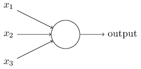
\begin{equation}output=\left\{\begin{matrix}0 & if\;\sum_i{w_ix_i} \le threshold \\ 1 & if\;\sum_i{w_ix_i} > threshold \end{matrix} \right . \label{perceptrons}\end{equation}

可以把感知机想象成一个带权投票机制，比如3位评委给一个歌手打分，打分分别为4分、1分、-3分，这3位评分的权重分别是1、3、2，则该歌手最终得分为$4*1+1*3+（-3）*2=1$。按大赛规则最终得分大于3时可晋级，所以最终$\sum_i{w_ix_i} < threshold, output=0$，该歌手被淘汰。

把上式换一种形式，用$-b$替换$threshold$：

\begin{equation}output=\left\{\begin{matrix}0 & if\;w\cdot x+b \le 0 \\ 1 & if\;w\cdot x+b > 0 \end{matrix} \right . \label{perceptrons2}\end{equation}

设置合适的w和b，一个感知机单元可以实现一个与非门（即先与后非）。

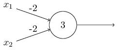
我们发现上面的感知机单元输入00时输出1；输入01时输出1；输入11时输出0。因为$0*(-2)+0*(-2)+3>0, 0*(-2)+1*(-2)+3>0, 1*(-2)+1*(-2)+3<0$。

用与非门可以实现任意复杂的逻辑电路，同理用感知机单元也可以实现任意复杂的决策系统。比如现实中的决策系统可能是这个样子的：

sigmoid单元

感知机单元的输出只有0和1，有时候w和b的微小变动可能就会导致输出截然相反。所以输出能不能是[0,1]上的实数概率值，而不要设成离散值{0,1}？其实直接用$w\cdot x$作为输出就已经是连续值了，但它不在区间[0,1]上，而sigmoid函数刚好可以把任意实数映射到[0,1]上。

神经元的输入

\begin{equation}z=\sum_i{w_ix_i}+b\label{input}\end{equation}

神经元的输出采用sigmoid激活函数

\begin{equation}\sigma(z)\equiv\frac{1}{1+e^{-z}}\label{active}\end{equation}

激活函数的导数

\begin{equation}\sigma(z)'=\frac{-1}{(1+e^{-z})^2}\cdot e^{-z}\cdot (-1)=\frac{1}{1+e^{-z}}\frac{e^{-z}}{1+e^{-z}}=\sigma(z)(1-\sigma(z))\label{ps}\end{equation}

能把任意实数映射到[0,1]的函数多得是，为什么偏偏选sigmoid函数呢？我认为主要是因为这个函数本身的数学性质为计算带来了方便，当然这里我们也可以给出其他解释。

学过概率论的同学都知道，累积分布函数cdf（cumulative distribution function）是概率密度函数pdf（probability density function）的积分，$cdf(u)$表示$x<u$的样本占总体的比例。对随机变量X施加cdf函数后$Y=cdf(X)$，随机变量$Y$服从[0,1]上的均匀分布。也就是说如果我们想把随机变量$X$归一化到[0,1]上，且归一化之后分布得很均匀，那么直接求$X$的累积分布函数即可。

粗略来看中心极限定理是说，如果一个随机变量是许多独立同分布的随机变量之和，那么它就近似服从正态分布。所以说正态分布是分布之王，当我们对一个随机变量全然不知时最保险的假设是它服从正态分布。正态分布的累积分布函数为

$$cdf(x)=\frac{1}{\sqrt{2\pi}\sigma}\int_{-\infty}^{x}{e^{-\frac{(t-\mu)^2}{2\sigma^2}}}dt$$

标准正态分布$\mu=0, \sigma=1$的累积分布函数图像为

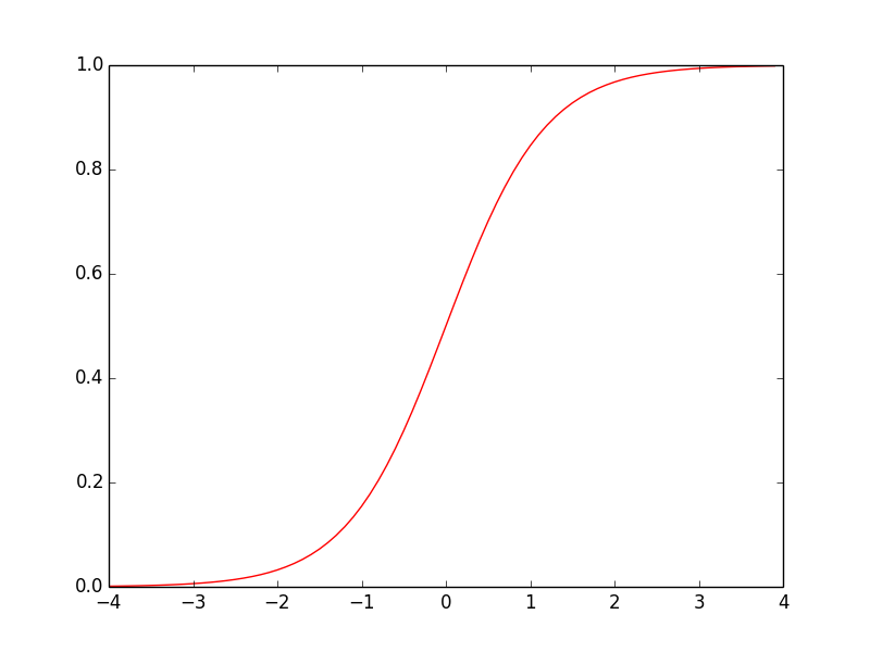
这和sigmoid函数图像极为相似，实际上标准正态分布的累积分布函数与$\sigma(x)=\frac{1}{1+e^{-1.7x}}$的吻合度非常高，如下图红线和绿线所示

以上就是选取sigmoid函数来作映射的缘由。

在有些情况下使用tanh激活函数会得到更好的效果。

$$tanh(z)=\frac{e^z-e^{-z}}{e^z+e^{-z}}$$

tanh的函数图像跟sigmoid很像，只是tanh的值域在[-1,1]。实际上sigmoid函数经过简单的平移缩放就能得到tanh函数：

$$\sigma(z)=\frac{1+tanh(\frac{z}{2})}{2}$$

根据分部求导法，先对分子求导，再对分母求导。

$$tanh'(z)=\frac{e^z+e^{-z}}{e^z+e^{-z}}-\frac{(e^z-e^{-z})(e^z-e^{-z})}{(e^z+e^{-z})^2}=1-tanh(z)^2$$

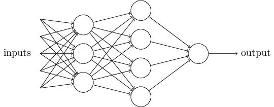
神经网络的结构

这里我们只介绍全连接神经网络，即第i层的每个神经元和第i-1层的每个神经元都有连接。

针对上图多说两句：输出层可以不止有1个神经元。隐藏层可以只有1层，也可以有多层。

每个神经元的输入和输出都遵循(\ref{input})式和(\ref{active})式。

只要一个输入层和一个输出层不行吗，为什么还搞出这么多隐藏层，弄得模型如此复杂、参数如此之多？其实没有原因，前人试出来这种结构好使罢了。不过还是可以跟大家分享一个“启发式”的想法，让大家加深对神经网络的理解。

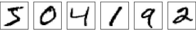
对于手写数字识别这个问题，每张图片由28*28=784个像素构成，每个像素取值{0，1}代表黑白。

我们可以设计这样一个神经网络：

输入层上的第个神经元对应一个像素。输出层有10个神经元，哪个神经元的输出值最大就认为图片上的数字是几。

我们可以想像隐藏层上的每个神经元各负责识别图片的一个局部特征，比如某个神经元只负责判断图片的局部是否为：

如果是，则该神经元就激活（即输出接近于1），否则就不激活（即输出接近于0）。同理隐藏层上的另外3个神经元分别负责判断图像的局部是否为

大家也看出来了，当图片同时满足这4个局部特征时，图像上的数字就是0，这也就是输出层起的作用。当隐藏层上的上述4个神经元都激活时，输出层上的第1个神经元就激活，即数字0对应的输出值会趋近于1。

我们还可以把网络结构设计成这样：

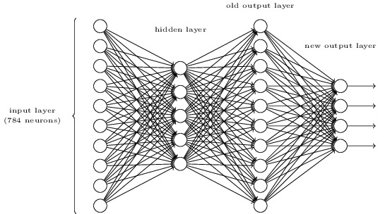
即上面所说的输出层变成了第2个隐藏层，额外加一个由4个神经元组成的输出层。为什么输出层有4个神经元呢？因为10个数字用4位二进制就可以表示，8=1000，9=1001，即当第2个隐藏层上数字8和数字9对应的神经元激活时，输出层上的首个神经元就应该激活。

那么问题来了，既然3层网络结构已经能够完成识别数字0-9的任务，为什么还要设计出一个4层网络结构呢？从试验结果上看，4层网络结构比3层的识别精度更高。这里同样我们给出一个“启发式”的原因，解释为什么要设计出更多的隐藏层：前面的隐藏层负责识别一些低级的特征（比如图像中的分界线），后面的隐藏层在此基础之上识别更高级更抽象的特征（比如图像中的拐角），最后输出层在表决时结论就越趋向于正确。

神经网络与奥卡姆剃刀原理背道而驰，奥卡姆老先生教导我们模型越简单、参数越少越好，而神经网络却是隐藏层越多预测的精度越高。当然后文会讲到神经网络中也需要引入正则化方法来防止过拟合，但这与设计更复杂的网络结构并不冲突。

正如感知机网络可以实现任意复杂的逻辑电路一样，只有一个隐藏层的神经网络就可以拟合任意复杂的连续函数，增加隐藏层个数或神经元个数可以提高拟合的精度。理论证明很复杂，但Michael Nielsen给出了可视化证明。

参数学习

每张图片都有一个期望输出$a$和实际输出$y(x)$，定义损失函数为

$$C(w,b)\equiv\frac{1}{2n}\sum_x{||y(x)-a||^2}$$

$n$是样本的个数。

基于梯度下降法

$$w_k\to w'_k=w_k-\eta\frac{\partial C}{\partial w_k}$$

$$b_l\to b'_l=b_l-\eta\frac{\partial C}{\partial b_l}$$

$\eta$是学习率。因为一共有$n$个样本，所以$w$和$b$最终怎么调整应该由这$n$个样本共同决定。

\begin{equation}\left\{\begin{matrix}w_k\to w'_k=w_k-\frac{\eta}{n}\sum_i{\frac{\partial C_{X_i}}{\partial w_k}} \\b_l\to b'_l=b_l-\frac{\eta}{n}\sum_i{\frac{\partial C_{X_i}}{\partial b_l}}\end{matrix}\right . \end{equation}

具体到神经网络中的每个权重$w_k$和每一个偏置$b_l$，$\frac{\partial C_{X_i}}{\partial w_k}$和$\frac{\partial C_{X_i}}{\partial b_l}$又该怎么求呢？根据导数的定义

$$f'(w)=lim_{\delta\to 0}\frac{f(w+\delta)-f(w)}{\delta}$$

这种方法计算量巨大，因为每调整一个参数$w_k$都要额外历经 一次完整的forward运算才能得到$f(w+\delta)$。我们最好通过解析式来求导。

\begin{equation}a^{l}_j = \sigma\left( \sum_k w^{l}_{jk} a^{l-1}_k + b^l_j \right)\label{active2}\end{equation}

$a^{l}_j $表示第$l$层上第$j$个神经元的输出，$w^{l}_{jk}$表示第$l-1$层上的第$k$个神经元到第$l$层上的第$j$个神经元之间的连接权重，$b^l_j$表示第$l$层上第$j$个神经元的偏置。

设神经网络的最后一层为第$L$层，只考虑1个样本的损失函数。

$$C=\frac{1}{2}\sum_j(y_j-a^L_j)^2$$

\begin{equation}\frac{\partial C}{\partial w_{jk}^L}=\frac{\partial C}{\partial a_j^L}\frac{\partial a_j^L}{\partial z_j^L}\frac{\partial z_j^L}{\partial w_{jk}^L}=(y_j-a_j^L)\sigma'(z_j^L)a_k^{L-1}\end{equation}

同理

\begin{equation}\frac{\partial C}{\partial b_j^L}=(y_j-a_j^L)\sigma'(z_j^L)\end{equation}

记\begin{equation}\delta_j^L=\frac{\partial C}{\partial a_j^L}\frac{\partial a_j^L}{\partial z_j^L}=\frac{\partial C}{\partial z_j^L}\end{equation}

则

\begin{equation}\frac{\partial C}{\partial w_{jk}^L}=\delta_j^L a_k^{L-1}\label{tag1}\end{equation}

\begin{equation}\frac{\partial C}{\partial b_j^L}=\delta_j^L\label{tag2}\end{equation}

\begin{equation}\delta_k^{L-1}=\frac{\partial C}{\partial z_k^{L-1}}=\sum_j\left(\frac{\partial C}{\partial z_j^L}\frac{\partial z_j^L}{\partial a_k^{L-1}}\frac{\partial a_k^{L-1}}{\partial z_k^{L-1}}\right)=\sum_j{\delta_j^L w_{jk}^L \sigma'(z_k^{L-1})}\label{tag3}\end{equation}

把$L$换成任意层$l(l>1)$，公式(\ref{tag1})(\ref{tag2})(\ref{tag3})依然成立。这样一次forward计算所有节点的输出，一次backpropagation调整所有的w和b，forward和backpropagation的时间复杂度是一样的，这是一种效果很高的学习算法。

numpy是python的一个矩阵运算库，在numpy中矩阵的加法是对应位置上的元素分别相加，矩阵的乘法是对应位置上的元素分别相乘（并不是做内积运算）。

>>> import numpy as np 
>>> a=np.array([2,4,8])
>>> b=np.array([1,3,5])
>>> print a+b 
[ 3  7 13]
>>> print a*b
[ 2 12 40]

(\ref{active2})式去掉下标$j$写成矩阵运算的形式

\begin{equation}a^{l}= \sigma(w^l\cdot a^{l-1}+ b^l)\end{equation}

$\cdot$是内积运算。

从github找了段神经网络的代码：

https://github.com/MichalDanielDobrzanski/DeepLearningPython35

"""network2.py
~~~~~~~~~~~~~~

An improved version of network.py, implementing the stochastic
gradient descent learning algorithm for a feedforward neural network.
Improvements include the addition of the cross-entropy cost function,
regularization, and better initialization of network weights.  Note
that I have focused on making the code simple, easily readable, and
easily modifiable.  It is not optimized, and omits many desirable
features.

"""

# Libraries
# Standard library
import json
import random
import sys

# Third-party libraries
import numpy as np


# Define the quadratic and cross-entropy cost functions

class QuadraticCost(object):

    @staticmethod
    def fn(a, y):
        """Return the cost associated with an output ``a`` and desired output
        ``y``.

        """
        return 0.5 * np.linalg.norm(a - y)**2

    @staticmethod
    def delta(z, a, y):
        """Return the error delta from the output layer."""
        return (a - y) * sigmoid_prime(z)


class CrossEntropyCost(object):

    @staticmethod
    def fn(a, y):
        """Return the cost associated with an output ``a`` and desired output
        ``y``.  Note that np.nan_to_num is used to ensure numerical
        stability.  In particular, if both ``a`` and ``y`` have a 1.0
        in the same slot, then the expression (1-y)*np.log(1-a)
        returns nan.  The np.nan_to_num ensures that that is converted
        to the correct value (0.0).

        """
        return np.sum(np.nan_to_num(-y * np.log(a) - (1 - y) * np.log(1 - a)))

    @staticmethod
    def delta(z, a, y):
        """Return the error delta from the output layer.  Note that the
        parameter ``z`` is not used by the method.  It is included in
        the method's parameters in order to make the interface
        consistent with the delta method for other cost classes.

        """
        return (a - y)


# Main Network class
class Network(object):

    def __init__(self, sizes, cost=CrossEntropyCost):
        """The list ``sizes`` contains the number of neurons in the respective
        layers of the network.  For example, if the list was [2, 3, 1]
        then it would be a three-layer network, with the first layer
        containing 2 neurons, the second layer 3 neurons, and the
        third layer 1 neuron.  The biases and weights for the network
        are initialized randomly, using
        ``self.default_weight_initializer`` (see docstring for that
        method).

        """
        self.num_layers = len(sizes)
        self.sizes = sizes
        self.default_weight_initializer()
        self.cost = cost

    def default_weight_initializer(self):
        """Initialize each weight using a Gaussian distribution with mean 0
        and standard deviation 1 over the square root of the number of
        weights connecting to the same neuron.  Initialize the biases
        using a Gaussian distribution with mean 0 and standard
        deviation 1.

        Note that the first layer is assumed to be an input layer, and
        by convention we won't set any biases for those neurons, since
        biases are only ever used in computing the outputs from later
        layers.

        """
        self.biases = [np.random.randn(y, 1) for y in self.sizes[1:]]
        self.weights = [np.random.randn(y, x) / np.sqrt(x)
                        for x, y in zip(self.sizes[:-1], self.sizes[1:])]

    def large_weight_initializer(self):
        """Initialize the weights using a Gaussian distribution with mean 0
        and standard deviation 1.  Initialize the biases using a
        Gaussian distribution with mean 0 and standard deviation 1.

        Note that the first layer is assumed to be an input layer, and
        by convention we won't set any biases for those neurons, since
        biases are only ever used in computing the outputs from later
        layers.

        This weight and bias initializer uses the same approach as in
        Chapter 1, and is included for purposes of comparison.  It
        will usually be better to use the default weight initializer
        instead.

        """
        self.biases = [np.random.randn(y, 1) for y in self.sizes[1:]]
        self.weights = [np.random.randn(y, x)
                        for x, y in zip(self.sizes[:-1], self.sizes[1:])]

    def feedforward(self, a):
        """Return the output of the network if ``a`` is input."""
        for b, w in zip(self.biases, self.weights):
            a = sigmoid(np.dot(w, a) + b)
        return a

    def SGD(self, training_data, epochs, mini_batch_size, eta,
            lmbda=0.0,
            evaluation_data=None,
            monitor_evaluation_cost=False,
            monitor_evaluation_accuracy=False,
            monitor_training_cost=False,
            monitor_training_accuracy=False):
        """Train the neural network using mini-batch stochastic gradient
        descent.  The ``training_data`` is a list of tuples ``(x, y)``
        representing the training inputs and the desired outputs.  The
        other non-optional parameters are self-explanatory, as is the
        regularization parameter ``lmbda``.  The method also accepts
        ``evaluation_data``, usually either the validation or test
        data.  We can monitor the cost and accuracy on either the
        evaluation data or the training data, by setting the
        appropriate flags.  The method returns a tuple containing four
        lists: the (per-epoch) costs on the evaluation data, the
        accuracies on the evaluation data, the costs on the training
        data, and the accuracies on the training data.  All values are
        evaluated at the end of each training epoch.  So, for example,
        if we train for 30 epochs, then the first element of the tuple
        will be a 30-element list containing the cost on the
        evaluation data at the end of each epoch. Note that the lists
        are empty if the corresponding flag is not set.

        """
        if evaluation_data:
            n_data = len(evaluation_data)
        n = len(training_data)
        evaluation_cost, evaluation_accuracy = [], []
        training_cost, training_accuracy = [], []
        for j in xrange(epochs):
            random.shuffle(training_data)
            mini_batches = [
                training_data[k:k + mini_batch_size]
                for k in xrange(0, n, mini_batch_size)]
            for mini_batch in mini_batches:
                self.update_mini_batch(
                    mini_batch, eta, lmbda, len(training_data))
            print "Epoch %s training complete" % j
            if monitor_training_cost:
                cost = self.total_cost(training_data, lmbda)
                training_cost.append(cost)
                print "Cost on training data: {}".format(cost)
            if monitor_training_accuracy:
                accuracy = self.accuracy(training_data, convert=True)
                training_accuracy.append(accuracy)
                print "Accuracy on training data: {} / {}".format(
                    accuracy, n)
            if monitor_evaluation_cost:
                cost = self.total_cost(evaluation_data, lmbda, convert=True)
                evaluation_cost.append(cost)
                print "Cost on evaluation data: {}".format(cost)
            if monitor_evaluation_accuracy:
                accuracy = self.accuracy(evaluation_data)
                evaluation_accuracy.append(accuracy)
                print "Accuracy on evaluation data: {} / {}".format(
                    self.accuracy(evaluation_data), n_data)
            print
        return evaluation_cost, evaluation_accuracy, \
            training_cost, training_accuracy

    def update_mini_batch(self, mini_batch, eta, lmbda, n):
        """Update the network's weights and biases by applying gradient
        descent using backpropagation to a single mini batch.  The
        ``mini_batch`` is a list of tuples ``(x, y)``, ``eta`` is the
        learning rate, ``lmbda`` is the regularization parameter, and
        ``n`` is the total size of the training data set.

        """
        nabla_b = [np.zeros(b.shape) for b in self.biases]
        nabla_w = [np.zeros(w.shape) for w in self.weights]
        for x, y in mini_batch:
            delta_nabla_b, delta_nabla_w = self.backprop(x, y)
            nabla_b = [nb + dnb for nb, dnb in zip(nabla_b, delta_nabla_b)]
            nabla_w = [nw + dnw for nw, dnw in zip(nabla_w, delta_nabla_w)]
        self.weights = [(1 - eta * (lmbda / n)) * w - (eta / len(mini_batch)) * nw
                        for w, nw in zip(self.weights, nabla_w)]
        self.biases = [b - (eta / len(mini_batch)) * nb
                       for b, nb in zip(self.biases, nabla_b)]

    def backprop(self, x, y):
        """Return a tuple ``(nabla_b, nabla_w)`` representing the
        gradient for the cost function C_x.  ``nabla_b`` and
        ``nabla_w`` are layer-by-layer lists of numpy arrays, similar
        to ``self.biases`` and ``self.weights``."""
        nabla_b = [np.zeros(b.shape) for b in self.biases]
        nabla_w = [np.zeros(w.shape) for w in self.weights]
        # feedforward
        activation = x
        activations = [x]  # list to store all the activations, layer by layer
        zs = []  # list to store all the z vectors, layer by layer
        for b, w in zip(self.biases, self.weights):
            z = np.dot(w, activation) + b
            zs.append(z)
            activation = sigmoid(z)
            activations.append(activation)
        # backward pass
        delta = (self.cost).delta(zs[-1], activations[-1], y)
        nabla_b[-1] = delta
        nabla_w[-1] = np.dot(delta, activations[-2].transpose())
        # Note that the variable l in the loop below is used a little
        # differently to the notation in Chapter 2 of the book.  Here,
        # l = 1 means the last layer of neurons, l = 2 is the
        # second-last layer, and so on.  It's a renumbering of the
        # scheme in the book, used here to take advantage of the fact
        # that Python can use negative indices in lists.
        for l in xrange(2, self.num_layers):
            z = zs[-l]
            sp = sigmoid_prime(z)
            delta = np.dot(self.weights[-l + 1].transpose(), delta) * sp
            nabla_b[-l] = delta
            nabla_w[-l] = np.dot(delta, activations[-l - 1].transpose())
        return (nabla_b, nabla_w)

    def accuracy(self, data, convert=False):
        """Return the number of inputs in ``data`` for which the neural
        network outputs the correct result. The neural network's
        output is assumed to be the index of whichever neuron in the
        final layer has the highest activation.

        The flag ``convert`` should be set to False if the data set is
        validation or test data (the usual case), and to True if the
        data set is the training data. The need for this flag arises
        due to differences in the way the results ``y`` are
        represented in the different data sets.  In particular, it
        flags whether we need to convert between the different
        representations.  It may seem strange to use different
        representations for the different data sets.  Why not use the
        same representation for all three data sets?  It's done for
        efficiency reasons -- the program usually evaluates the cost
        on the training data and the accuracy on other data sets.
        These are different types of computations, and using different
        representations speeds things up.  More details on the
        representations can be found in
        mnist_loader.load_data_wrapper.

        """
        if convert:
            results = [(np.argmax(self.feedforward(x)), np.argmax(y))
                       for (x, y) in data]
        else:
            results = [(np.argmax(self.feedforward(x)), y)
                       for (x, y) in data]
        return sum(int(x == y) for (x, y) in results)

    def total_cost(self, data, lmbda, convert=False):
        """Return the total cost for the data set ``data``.  The flag
        ``convert`` should be set to False if the data set is the
        training data (the usual case), and to True if the data set is
        the validation or test data.  See comments on the similar (but
        reversed) convention for the ``accuracy`` method, above.
        """
        cost = 0.0
        for x, y in data:
            a = self.feedforward(x)
            if convert:
                y = vectorized_result(y)
            cost += self.cost.fn(a, y) / len(data)
        cost += 0.5 * (lmbda / len(data)) * sum(
            np.linalg.norm(w)**2 for w in self.weights)
        return cost

    def save(self, filename):
        """Save the neural network to the file ``filename``."""
        data = {"sizes": self.sizes,
                "weights": [w.tolist() for w in self.weights],
                "biases": [b.tolist() for b in self.biases],
                "cost": str(self.cost.__name__)}
        f = open(filename, "w")
        json.dump(data, f)
        f.close()


if __name__ == '__main__':
    # weights = np.array([[1, 2, 3], [4, 5, 6]])
    # biases = np.array([[3], [8]])
    # data = {"sizes": [3, 3],
    #         "weights": [w.tolist() for w in weights],
    #         "biases": [b.tolist() for b in biases],
    #         "cost": str(CrossEntropyCost.__name__)}
    # cost = getattr(sys.modules[__name__], data["cost"])
    # print cost.__name__
    # print data
    import mnist_loader
    training_data, validation_data, test_data = mnist_loader.load_data_wrapper()
    net = Network([784, 30, 10])
    net.SGD(training_data, 30, 10, 3.0, evaluation_data=validation_data)

# Loading a Network


def load(filename):
    """Load a neural network from the file ``filename``.  Returns an
    instance of Network.

    """
    f = open(filename, "r")
    data = json.load(f)
    f.close()
    cost = getattr(sys.modules[__name__], data["cost"])
    net = Network(data["sizes"], cost=cost)
    net.weights = [np.array(w) for w in data["weights"]]
    net.biases = [np.array(b) for b in data["biases"]]
    return net

# Miscellaneous functions


def vectorized_result(j):
    """Return a 10-dimensional unit vector with a 1.0 in the j'th position
    and zeroes elsewhere.  This is used to convert a digit (0...9)
    into a corresponding desired output from the neural network.

    """
    e = np.zeros((10, 1))
    e[j] = 1.0
    return e


def sigmoid(z):
    """The sigmoid function."""
    return 1.0 / (1.0 + np.exp(-z))


def sigmoid_prime(z):
    """Derivative of the sigmoid function."""
    return sigmoid(z) * (1 - sigmoid(z))