


Python自然语言处理学习笔记(53):决策树
6.4 Decision Trees 决策树
In the next three sections, we'll take a closer look at three machine learning methods that can be used to automatically build classification models: decision trees, naive Bayes classifiers, and Maximum Entropy classifiers. As we've seen, it's possible to treat these learning methods as black boxes, simply training models and using them for prediction without understanding how they work. But there's a lot to be learned from taking a closer look at how these learning methods select models based on the data in a training set. An understanding of these methods can help guide our selection of appropriate features, and especially our decisions about how those features should be encoded. And an understanding of the generated models can allow us to extract information about which features are most informative, and how those features relate to one another.
A decision tree is a simple flowchart that selects labels for input values. This flowchart consists of decision nodes(决策节点), which check feature values, and leaf nodes, which assign labels. To choose the label for an input value, we begin at the flowchart's initial decision node, known as its root node. This node contains a condition that checks one of the input value's features, and selects a branch based on that feature's value. Following the branch that describes our input value, we arrive at a new decision node, with a new condition on the input value's features. We continue following the branch selected by each node's condition, until we arrive at a leaf node which provides a label for the input value. Figure 6.11 shows an example decision tree model for the name gender task.
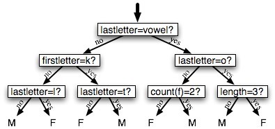
Figure 6.11: Decision Tree model for the name gender task. Note that tree diagrams are conventionally drawn "upside down,(倒置)" with the root at the top, and the leaves at the bottom.
Once we have a decision tree, it is straightforward to use it to assign labels to new input values. What's less straightforward is how we can build a decision tree that models a given training set. But before we look at the learning algorithm for building decision trees, we'll consider a simpler task: picking the best "decision stump"(决策树桩) for a corpus. A decision stump is a decision tree with a single node that decides how to classify inputs based on a single feature. It contains one leaf for each possible feature value, specifying the class label that should be assigned to inputs whose features have that value. In order to build a decision stump, we must first decide which feature should be used. The simplest method is to just build a decision stump for each possible feature, and see which one achieves the highest accuracy on the training data, although there are other alternatives that we will discuss below. Once we've picked a feature, we can build the decision stump by assigning a label to each leaf based on the most frequent label for the selected examples in the training set (i.e., the examples where the selected feature has that value).
Given the algorithm for choosing decision stumps, the algorithm for growing larger decision trees is straightforward. We begin by selecting the overall best decision stump for the classification task. We then check the accuracy of each of the leaves on the training set. Leaves that do not achieve sufficient accuracy are then replaced by new decision stumps, trained on the subset of the training corpus that is selected by the path to the leaf. For example, we could grow the decision tree in Figure 6.11 by replacing the leftmost leaf with a new decision stump, trained on the subset of the training set names that do not start with a "k" or end with a vowel(元音) or an "l."
Entropy and Information Gain 熵和信息增益
As was mentioned before, there are several methods for identifying the most informative feature for a decision stump. One popular alternative, called information gain, measures how much more organized the input values become when we divide them up using a given feature. To measure how disorganized the original set of input values are, we calculate entropy of their labels, which will be high if the input values have highly varied labels, and low if many input values all have the same label. In particular, entropy is defined as the sum of the probability of each label times the log probability of that same label(熵定义为每个label的概率乘以同个label的概率值对数之和,加负号是因为小于1的对数为负):
| (1) |
| H = −Σl |in| labelsP(l) × log2P(l). |
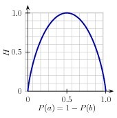
Figure 6.12: The entropy of labels in the name gender prediction task, as a function of the percentage of names in a given set that are male.
For example, Figure 6.12 shows how the entropy of labels in the name gender prediction task depends on the ratio of male to female names. Note that if most input values have the same label (e.g., if P(male) is near 0 or near 1), then entropy is low. In particular, labels that have low frequency do not contribute much to the entropy (since P(l) is small), and labels with high frequency also do not contribute much to the entropy (since log2P(l) is small). On the other hand, if the input values have a wide variety of labels, then there are many labels with a "medium" frequency, where neither P(l) nor log2P(l) is small, so the entropy is high. Example 6.13 demonstrates how to calculate the entropy of a list of labels.
| ||
| ||
| Example 6.13 (code_entropy.py): Calculating the Entropy of a List of Labels |
Once we have calculated the entropy of the original set of input values' labels, we can determine how much more organized the labels become once we apply the decision stump. To do so, we calculate the entropy for each of the decision stump's leaves, and take the average of those leaf entropy values (weighted by the number of samples in each leaf). The information gain is then equal to the original entropy minus this new, reduced entropy. The higher the information gain, the better job the decision stump does of dividing the input values into coherent groups, so we can build decision trees by selecting the decision stumps with the highest information gain.(不太理解。有了些理解,查看了决策树和ID3算法,明白了其原理就是按照信息增益越大的靠近根节点进行分类)
Another consideration for decision trees is efficiency. The simple algorithm for selecting decision stumps described above must construct a candidate decision stump for every possible feature, and this process must be repeated for every node in the constructed decision tree. A number of algorithms have been developed to cut down(减少) on the training time by storing and reusing information about previously evaluated examples.
Decision trees have a number of useful qualities. To begin with, they're simple to understand, and easy to interpret. This is especially true near the top of the decision tree, where it is usually possible for the learning algorithm to find very useful features. Decision trees are especially well suited to cases where many hierarchical categorical distinctions(有层次的分类的区别) can be made. For example, decision trees can be very effective at capturing phylogeny trees(系统树).
However, decision trees also have a few disadvantages. One problem is that, since each branch in the decision tree splits the training data, the amount of training data available to train nodes lower in the tree can become quite small. As a result, these lower decision nodes may overfit the training set, learning patterns that reflect idiosyncrasies(风格) of the training set rather than linguistically significant patterns in the underlying problem. One solution to this problem is to stop dividing nodes once the amount of training data becomes too small. Another solution is to grow a full decision tree, but then to prune(修枝) decision nodes that do not improve performance on a dev-test.
A second problem with decision trees is that they force features to be checked in a specific order, even when features may act relatively independently of one another. For example, when classifying documents into topics (such as sports, automotive, or murder mystery), features such as hasword(football) are highly indicative of a specific label, regardless of what other the feature values are. Since there is limited space near the top of the decision tree, most of these features will need to be repeated on many different branches in the tree. And since the number of branches increases exponentially as we go down the tree, the amount of repetition can be very large.
A related problem is that decision trees are not good at making use of features that are weak predictors of the correct label. Since these features make relatively small incremental improvements, they tend to occur very low in the decision tree. But by the time the decision tree learner has descended far enough to use these features, there is not enough training data left to reliably determine what effect they should have. If we could instead look at the effect of these features across the entire training set, then we might be able to make some conclusions about how they should affect the choice of label.
The fact that decision trees require that features be checked in a specific order limits their ability to exploit features that are relatively independent of one another. The naive Bayes classification method, which we'll discuss next, overcomes this limitation by allowing all features to act "in parallel."

 浙公网安备 33010602011771号