Python自然语言处理学习笔记(50)： 监督式分类

Chapter6   

Learning to Classify Text 学习文本分类

Detecting patterns is a central part of Natural Language Processing(模式检测是自然语言处理的核心内容). Words ending in -ed tend to be past tense verbs (Chapter 5). Frequent use of will is indicative of news text (Chapter 3). These observable patterns — word structure and word frequency — happen to correlate with particular aspects of meaning, such as tense and topic(时态和主题). But how did we know where to start looking, which aspects of form to associate with which aspects of meaning?

The goal of this chapter is to answer the following questions:

   本章的学习目标是用来回答以下问题： 

1. How can we identify particular features of language data that are salient for classifying it?

我们如何识别语言数据的特有性质来对它们进行明显地分类？

2. How can we construct models of language that can be used to perform language processing tasks automatically?

我们该如何构建可以用于自动地执行语言处理任务的语言模型？

3. What can we learn about language from these models?

从这些模型我们可以学到哪些语言知识？

Along the way we will study some important machine learning techniques, including decision trees, naive Bayes' classifiers, and maximum entropy classifiers. We will gloss over（掩盖） the mathematical and statistical underpinnings（基础） of these techniques, focusing instead on how and when to use them (see the Further Readings section for more technical background). Before looking at these methods, we first need to appreciate（领会） the broad scope of this topic.

沿着这个方向，我们将学习一些重要的机器学习技术，包含了决策数，朴素贝叶斯分类器，最大熵分类器。我们将掩盖这些技术的数学和统计基础，集中于如何并且何时去使用它们。你可以浏览深入阅读章节来了解更多的技术背景知识。在学习这些方法前，我们首先要领会到这一主题的广泛的范围。 

 

6.1   Supervised Classification 监督式分类

Classification is the task of choosing the correct class label（类别标签） for a given input. In basic classification tasks, each input is considered in isolation from all other inputs, and the set of labels is defined in advance. Some examples of classification tasks are:

• Deciding whether an email is spam or not.

判断电子邮件是否为垃圾邮件。

• Deciding what the topic of a news article is, from a fixed list of topic areas such as "sports," "technology," and "politics."

判断新闻报道的主题是什么，从固定的列表主题领域诸如"sports," "technology," 以及"politics."

• Deciding whether a given occurrence of the word bank is used to refer to a river bank, a financial institution, the act of tilting to the side, or the act of depositing something in a financial institution.

判断给定的出现单词bank是否用于指的是river bank（河岸），金融机构，倾斜到一边的行为，或者是在金融机构里存储的行为。

The basic classification task has a number of interesting variants. For example, in multi-class classification, each instance may be assigned multiple labels; in open-class classification, the set of labels is not defined in advance; and in sequence classification, a list of inputs are jointly（共同地） classified.

A classifier is called supervised if it is built based on training corpora containing the correct label for each input. The framework used by supervised classification is shown in Figure 6.1.一个分类器被称为是监督式的，如果它是建立在基于包含了每个输入的正确标注的训练语料库上。

 

 

 

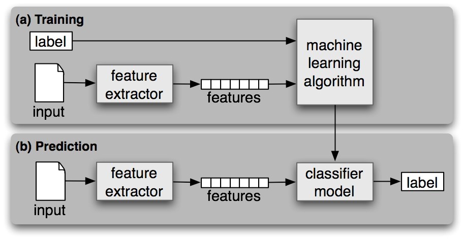
Figure 6.1: Supervised Classification. (a) During training, a feature extractor（特征提取器） is used to convert each input value to a feature set. These feature sets, which capture the basic information about each input that should be used to classify it, are discussed in the next section. Pairs of feature sets and labels are fed into（被送入） the machine learning algorithm to generate a model. (b) During prediction, the same feature extractor is used to convert unseen inputs to feature sets. These feature sets are then fed into the model, which generates predicted labels.

In the rest of this section, we will look at how classifiers can be employed to solve a wide variety of tasks. Our discussion is not intended to be comprehensive（全面的）, but to give a representative sample of tasks that can be performed with the help of text classifiers.

 

Gender Identification 性别鉴定

In Section 2.4 we saw that male and female names have some distinctive characteristics. Names ending in a, e and i are likely to be female, while names ending in k, o, r, s and t are likely to be male(名字以a,e,i结尾的可能是女性，而以k,or,s,t结尾的可能是男性。看看英文的性别多分明啊，我这有个叫白雪的男童鞋！...). Let's build a classifier to model these differences more precisely.

The first step in creating a classifier is deciding what features of the input are relevant, and how to encode those features.(创建分类器的第一步是决定输入的哪些特征是相关的，并且如何编码这些特征。)For this example, we'll start by just looking at the final letter of a given name. The following feature extractor function builds a dictionary containing relevant information about a given name:

>>> def gender_features(word): ...     return {'last_letter': word[-1]} >>> gender_features('Shrek') {'last_letter': 'k'}

The returned dictionary, known as a feature set（特征集）, maps from features' names to their values. Feature names are case-sensitive strings that typically provide a short human-readable description of the feature. Feature values are values with simple types, such as booleans, numbers, and strings.

Note：Most classification methods require that features be encoded using simple value types, such as booleans, numbers, and strings. But note that just because a feature has a simple type, does not necessarily mean that the feature's value is simple to express or compute; indeed, it is even possible to use very complex and informative values, such as the output of a second supervised classifier, as features.
注意：大多数分类方法需要使用简单的值类型将特征编码，例如布尔值，数值，字符串。但是注意这只是因为特征有一个简单的类型，并不意味着特征的值也需要简单地表示或者计算；确实，特征值甚至可能使用非常复杂和信息性的值，比如第二个监督式分类器的输出作为特征。

Now that we've defined a feature extractor, we need to prepare a list of examples and corresponding class labels.

>>> from nltk.corpus import names >>> import random >>> names = ([(name, 'male') for name in names.words('male.txt')] + ...          [(name, 'female') for name in names.words('female.txt')]) >>> import random >>> random.shuffle(names)

Next, we use the feature extractor to process the names data, and divide the resulting list of feature sets into a training set and a test set.(下一步我们使用特征提取器来处理名字数据，并且将特征列表分为训练集合和测试集合。) The training set is used to train a new "naive Bayes" classifier.

>>> featuresets = [(gender_features(n), g) for (n,g) in names] >>> train_set, test_set = featuresets[500:], featuresets[:500] >>> classifier = nltk.NaiveBayesClassifier.train(train_set)

We will learn more about the naive Bayes classifier later in the chapter. For now, let's just test it out on some names that did not appear in its training data:

>>> classifier.classify(gender_features('Neo')) 'male' >>> classifier.classify(gender_features('Trinity')) 'female'

Observe that these character names from The Matrix(黑客帝国) are correctly classified(看看那些来自于黑客帝国的名字也能被正确地划分，老外真搞...). Although this science fiction movie is set in 2199, it still conforms with our expectations about names and genders. We can systematically evaluate the classifier on a much larger quantity of unseen data:

>>> print nltk.classify.accuracy(classifier, test_set) 0.758

Finally, we can examine the classifier to determine which features it found most effective for distinguishing the names' genders:

（最后，我们可以检查这些分类器来决定查找到的特征集合中可以最有效地区分名字的性别） 

>>> classifier.show_most_informative_features(5) Most Informative Features    last_letter = 'a'             female : male  =   38.3 : 1.0     last_letter = 'k'             male : female =     31.4 : 1.0     last_letter = 'f'             male : female =     15.3 : 1.0     last_letter = 'p'             male : female =     10.6 : 1.0     last_letter = 'w'              male : female =     10.6 : 1.0

This listing shows that the names in the training set that end in "a" are female 38 times more often than they are male, but names that end in "k" are male 31 times more often than they are female. These ratios are known as likelihood ratios（似然率）, and can be useful for comparing different feature-outcome relationships.

Note

Your Turn: Modify the gender_features() function to provide the classifier with features encoding the length of the name, its first letter, and any other features that seem like they might be informative. Retrain the classifier with these new features, and test its accuracy.

When working with large corpora, constructing a single list that contains the features of every instance can use up a large amount of memory. In these cases, use the function nltk.classify.apply_features, which returns an object that acts like a list but does not store all the feature sets in memory(但是没有把所有的特征集存入内存):

>>> from nltk.classify import apply_features >>> train_set = apply_features(gender_features, names[500:]) >>> test_set = apply_features(gender_features, names[:500])

 

Choosing The Right Features 选择正确的特征

Selecting relevant features and deciding how to encode them for a learning method can have an enormous impact on the learning method's ability to extract a good model. Much of the interesting work in building a classifier is deciding what features might be relevant, and how we can represent them. Although it's often possible to get decent(相当好的) performance by using a fairly simple and obvious set of features, there are usually significant gains to be had by using carefully constructed features based on a thorough understanding of the task at hand（眼前）.

Typically, feature extractors are built through a process of trial-and-error（反复实验法）, guided by intuitions about what information is relevant to the problem. It's common to start with a "kitchen sink"（厨房水槽） approach, including all the features that you can think of, and then checking to see which features actually are helpful. We take this approach for name gender features in Example 6.2.

def gender_features2(name):     features = {}    features["firstletter"] = name[0].lower()     features["lastletter"] = name[-1].lower()     for letter in 'abcdefghijklmnopqrstuvwxyz':         features["count(%s)" % letter] = name.lower().count(letter)         features["has(%s)" % letter] = (letter in name.lower())     return features

>>> gender_features2('John') {'count(j)': 1, 'has(d)': False, 'count(b)': 0, ...}

Example 6.2 (code_gender_features_overfitting.py):  The featuresets returned by this feature extractor contain a large number of specific features, leading to overfitting（过度适合） for the relatively small Names Corpus.

 

However, there are usually limits to the number of features that you should use with a given learning algorithm — if you provide too many features, then the algorithm will have a higher chance of relying on（依赖） idiosyncrasies（风格） of your training data that don't generalize well to new examples. This problem is known as overfitting, and can be especially problematic when working with small training sets. For example, if we train a naive Bayes classifier using the feature extractor shown in Example 6.2, it will overfit relatively small training set, resulting in a system whose accuracy is about 1% lower than the accuracy of a classifier that only pays attention to the final letter of each name:

>>> featuresets = [(gender_features2(n), g) for (n,g) in names] >>> train_set, test_set = featuresets[500:], featuresets[:500] >>> classifier = nltk.NaiveBayesClassifier.train(train_set) >>> print nltk.classify.accuracy(classifier, test_set) 0.748

Once an initial set of features has been chosen, a very productive method for refining the feature set is error analysis（错误分析）. First, we select a development set（开发集合，包含了创建该模型的语料库数据）, containing the corpus data for creating the model. This development set is then subdivided into the training set and the dev-test set.

>>> train_names = names[1500:] >>> devtest_names = names[500:1500] >>> test_names = names[:500]

The training set is used to train the model, and the dev-test set is used to perform error analysis. The test set serves in our final evaluation of the system. For reasons discussed below, it is important that we employ a separate dev-test set for error analysis, rather than just using the test set. The division of the corpus data into different subsets is shown in Figure 6.3.

 

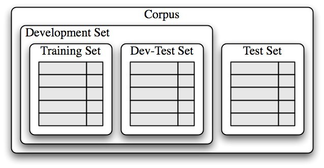
Figure 6.3: Organization of corpus data for training supervised classifiers. The corpus data is divided into two sets: the development set, and the test set. The development set is often further subdivided into a training set and a dev-test set.用于训练监督式分类器的语料库数据的组织结构。语料库数据被划分为两个集合：开发集合与测试集合。开放集合常常被进一步划分为训练集合与开发测试集合。

Having divided the corpus into appropriate datasets, we train a model using the training set , and then run it on the devtest set.

>>> train_set = [(gender_features(n), g) for (n,g) in train_names] >>> devtest_set = [(gender_features(n), g) for (n,g) in devtest_names] >>> test_set = [(gender_features(n), g) for (n,g) in test_names] >>> classifier = nltk.NaiveBayesClassifier.train(train_set) >>> print nltk.classify.accuracy(classifier, devtest_set) 0.765

Using the dev-test set, we can generate a list of the errors that the classifier makes when predicting name genders:

>>> errors = [] >>> for (name, tag) in devtest_names: ...     guess = classifier.classify(gender_features(name)) ...     if guess != tag: ...         errors.append( (tag, guess, name) )

We can then examine individual error cases where the model predicted the wrong label, and try to determine what additional pieces of information would allow it to make the right decision (or which existing pieces of information are tricking it into making the wrong decision). The feature set can then be adjusted accordingly. The names classifier that we have built generates about 100 errors on the dev-test corpus:

>>> for (tag, guess, name) in sorted(errors): ...     print 'correct=%-8s guess=%-8s name=%-30s' % (tag, guess, name)  ... correct=female   guess=male     name=Cindelyn  ... correct=female   guess=male     name=Katheryn correct=female   guess=male     name=Kathryn  ... correct=male     guess=female   name=Aldrich  ... correct=male     guess=female   name=Mitch  ... correct=male     guess=female   name=Rich  ...

Looking through this list of errors makes it clear that some suffixes that are more than one letter can be indicative of name genders. For example, names ending in yn appear to be predominantly female, despite the fact that names ending in n tend to be male; and names ending in ch are usually male, even though names that end in h tend to be female. We therefore adjust our feature extractor to include features for two-letter suffixes:

>>> def gender_features(word): ...     return {'suffix1': word[-1:], ...             'suffix2': word[-2:]}

Rebuilding the classifier with the new feature extractor, we see that the performance on the dev-test dataset improves by almost 3 percentage points (from 76.5% to 78.2%):

>>> train_set = [(gender_features(n), g) for (n,g) in train_names] >>> devtest_set = [(gender_features(n), g) for (n,g) in devtest_names] >>> classifier = nltk.NaiveBayesClassifier.train(train_set) >>> print nltk.classify.accuracy(classifier, devtest_set) 0.782

This error analysis procedure can then be repeated, checking for patterns in the errors that are made by the newly improved classifier. Each time the error analysis procedure is repeated, we should select a different dev-test/training split, to ensure that the classifier does not start to reflect idiosyncrasies in the dev-test set.

But once we've used the dev-test set to help us develop the model, we can no longer trust that it will give us an accurate idea of how well the model would perform on new data. It is therefore important to keep the test set separate, and unused（确保测试数据独立未使用的）, until our model development is complete. At that point, we can use the test set to evaluate well our model will perform on new input values.

 

Document Classification 文本分类

 

In Section 2.1, we saw several examples of corpora where documents have been labeled with categories. Using these corpora, we can build classifiers that will automatically tag new documents with appropriate category labels. First, we construct a list of documents, labeled with the appropriate categories. For this example, we've chosen the Movie Reviews Corpus, which categorizes each review as positive or negative.这个例子中，我们选择了电影评论语料库，该语料库按照正面和负面评论进行了分类。

>>> from nltk.corpus import movie_reviews >>> documents = [(list(movie_reviews.words(fileid)), category) ...              for category in movie_reviews.categories() ...              for fileid in movie_reviews.fileids(category)] >>> random.shuffle(documents)

Next, we define a feature extractor for documents, so the classifier will know which aspects of the data it should pay attention to (Example 6.4). For document topic identification, we can define a feature for each word, indicating whether the document contains that word. To limit the number of features that the classifier needs to process, we begin by constructing a list of the 2000 most frequent words in the overall corpus. We can then define a feature extractor that simply checks whether each of these words is present in a given document.

all_words = nltk.FreqDist(w.lower() for w in movie_reviews.words()) word_features = all_words.keys()[:2000] def document_features(document):     document_words = set(document)     features = {}     for word in word_features:         features['contains(%s)' % word] = (word in document_words)     return features

>>> print document_features(movie_reviews.words('pos/cv957_8737.txt')) {'contains(waste)': False, 'contains(lot)': False, ...}

Note

The reason that we compute the set of all words in a document in, rather than just checking if word in document, is that checking whether a word occurs in a set is much faster than checking whether it occurs in a list (Section 4.7).

Now that we've defined our feature extractor, we can use it to train a classifier to label new movie reviews (Example 6.5). To check how reliable the resulting classifier is, we compute its accuracy on the test set. And once again, we can use show_most_informative_features() to find out which features the classifier found to be most informative.

featuresets = [(document_features(d), c) for (d,c) in documents] train_set, test_set = featuresets[100:], featuresets[:100] classifier = nltk.NaiveBayesClassifier.train(train_set)

>>> print nltk.classify.accuracy(classifier, test_set) 0.81 >>> classifier.show_most_informative_features(5) Most Informative Features    contains(outstanding) = True     pos : neg    =     11.1 : 1.0    contains(seagal) = True         neg : pos    =      7.7 : 1.0    contains(wonderfully) = True    pos : neg    =      6.8 : 1.0    contains(damon) = True         pos : neg    =      5.9 : 1.0    contains(wasted) = True         neg : pos    =      5.8 : 1.0

Example 6.5 (code_document_classify_use.py):

Apparently（显然地） in this corpus, a review that mentions "Seagal" is almost 8 times more likely to be negative than positive, while a review that mentions "Damon" is about 6 times more likely to be positive.

 

Part-of-Speech Tagging 词性标注

In Chapter 5 we built a regular expression tagger that chooses a part-of-speech tag for a word by looking at the internal make-up（内部构造） of the word. However, this regular expression tagger had to be hand-crafted（手工制作的）. Instead, we can train a classifier to work out which suffixes are most informative. Let's begin by finding out what the most common suffixes are:

>>> from nltk.corpus import brown >>> suffix_fdist = nltk.FreqDist() >>> for word in brown.words(): ...     word = word.lower() ...     suffix_fdist.inc(word[-1:]) ...     suffix_fdist.inc(word[-2:]) ...     suffix_fdist.inc(word[-3:])

>>> common_suffixes = suffix_fdist.keys()[:100] >>> print common_suffixes ['e', ',', '.', 's', 'd', 't', 'he', 'n', 'a', 'of', 'the',  'y', 'r', 'to', 'in', 'f', 'o', 'ed', 'nd', 'is', 'on', 'l',  'g', 'and', 'ng', 'er', 'as', 'ing', 'h', 'at', 'es', 'or',  're', 'it', '``', 'an', "''", 'm', ';', 'i', 'ly', 'ion', ...]

Next, we'll define a feature extractor function which checks a given word for these suffixes:

>>> def pos_features(word): ...     features = {} ...     for suffix in common_suffixes: ...       features['endswith(%s)' % suffix] = word.lower().endswith(suffix) ...     return features

Feature extraction functions behave like tinted glasses（有色眼镜）, highlighting some of the properties (colors) in our data and making it impossible to see other properties. The classifier will rely exclusively on these highlighted properties when determining how to label inputs. In this case, the classifier will make its decisions based only on information about which of the common suffixes (if any) a given word has.

Now that we've defined our feature extractor, we can use it to train a new "decision tree" classifier (to be discussed in Section 6.4):

>>> tagged_words = brown.tagged_words(categories='news') >>> featuresets = [(pos_features(n), g) for (n,g) in tagged_words]

>>> size = int(len(featuresets) * 0.1) >>> train_set, test_set = featuresets[size:], featuresets[:size]

>>> classifier = nltk.DecisionTreeClassifier.train(train_set) >>> nltk.classify.accuracy(classifier, test_set) 0.62705121829935351

>>> classifier.classify(pos_features('cats')) 'NNS'

One nice feature of decision tree models is that they are often fairly easy to interpret — we can even instruct NLTK to print them out as pseudocode:

>>> print classifier.pseudocode(depth=4) if endswith(,) == True: return ',' if endswith(,) == False:  if endswith(the) == True: return 'AT'  if endswith(the) == False:     if endswith(s) == True:       if endswith(is) == True: return 'BEZ'       if endswith(is) == False: return 'VBZ'     if endswith(s) == False:       if endswith(.) == True: return '.'       if endswith(.) == False: return 'NN'

Here, we can see that the classifier begins by checking whether a word ends with a comma — if so, then it will receive the special tag ",". Next, the classifier checks if the word ends in "the", in which case it's almost certainly a determiner. This "suffix" gets used early by the decision tree because the word "the" is so common. Continuing on, the classifier checks if the word ends in "s". If so, then it's most likely to receive the verb tag VBZ (unless it's the word "is", which has a special tag BEZ), and if not, then it's most likely a noun (unless it's the punctuation mark "."). The actual classifier contains further nested if-then statements below the ones shown here, but the depth=4 argument just displays the top portion（顶端部分） of the decision tree.

 

Exploiting Context 语境探索

By augmenting the feature extraction function, we could modify this part-of-speech tagger to leverage（影响） a variety of other word-internal features, such as the length of the word, the number of syllables it contains, or its prefix. However, as long as the feature extractor just looks at the target word, we have no way to add features that depend on the context that the word appears in. But contextual features often provide powerful clues about the correct tag — for example, when tagging the word "fly," knowing that the previous word is "a" will allow us to determine that it is functioning as a noun, not a verb.

In order to accommodate features that depend on a word's context, we must revise the pattern that we used to define our feature extractor. Instead of just passing in the word to be tagged, we will pass in a complete (untagged) sentence, along with the index of the target word(我们将会传递一个完整（未标记的）的句子，带有目标单词的索引). This approach is demonstrated in Example 6.6, which employs a context-dependent feature extractor to define a part of speech tag classifier.

def pos_features(sentence, i):     features = {"suffix(1)": sentence[i][-1:],                 "suffix(2)": sentence[i][-2:],                 "suffix(3)": sentence[i][-3:]}     if i == 0:         features["prev-word"] = "<START>"     else:         features["prev-word"] = sentence[i-1]     return features

>>> pos_features(brown.sents()[0], 8) {'suffix(3)': 'ion', 'prev-word': 'an', 'suffix(2)': 'on', 'suffix(1)': 'n'}   >>> tagged_sents = brown.tagged_sents(categories='news') >>> featuresets = [] >>> for tagged_sent in tagged_sents: ...     untagged_sent = nltk.tag.untag(tagged_sent) ...     for i, (word, tag) in enumerate(tagged_sent): ...         featuresets.append( (pos_features(untagged_sent, i), tag) )   >>> size = int(len(featuresets) * 0.1) >>> train_set, test_set = featuresets[size:], featuresets[:size] >>> classifier = nltk.NaiveBayesClassifier.train(train_set)   >>> nltk.classify.accuracy(classifier, test_set) 0.78915962207856782

Example 6.6 (code_suffix_pos_tag.py):

Figure 6.6: A part-of-speech classifier whose feature detector examines the context in which a word appears in order to determine which part of speech tag should be assigned. In particular, the identity of the previous word is included as a feature.

 

It’s clear that exploiting contextual features improves the performance of our part-of-speech tagger. For example, the classifier learns that a word is likely to be a noun if it comes immediately after the word "large" or the word "gubernatorial". However, it is unable to learn the generalization that a word is probably a noun if it follows an adjective, because it doesn't have access to the previous word's part-of-speech tag. In general, simple classifiers always treat each input as independent from all other inputs. In many contexts, this makes perfect sense. For example, decisions about whether names tend to be male or female can be made on a case-by-case（具体分析） basis. However, there are often cases, such as part-of-speech tagging, where we are interested in solving classification problems that are closely related to one another.

 

Sequence Classification 序列分类

In order to capture the dependencies between related classification tasks, we can use joint classifier models（联合分类器模型）, which choose an appropriate labeling for a collection of related inputs. In the case of part-of-speech tagging, a variety of different sequence classifier models（序列分类器模型） can be used to jointly choose part-of-speech tags for all the words in a given sentence.

One sequence classification strategy, known as consecutive classification （一致性分类）or greedy sequence classification（贪婪序列分类）, is to find the most likely class label for the first input, then to use that answer to help find the best label for the next input. The process can then be repeated until all of the inputs have been labeled. This is the approach that was taken by the bigram tagger from Section 5.5, which began by choosing a part-of-speech tag for the first word in the sentence, and then chose the tag for each subsequent word based on the word itself and the predicted tag for the previous word.

This strategy is demonstrated in Example 6.7. First, we must augment our feature extractor function to take a history argument, which provides a list of the tags that we've predicted for the sentence so far. Each tag in history corresponds with a word in sentence（在历史中的每个标记对应中句子中的单词）. But note that history will only contain tags for words we've already classified, that is, words to the left of the target word. Thus, while it is possible to look at some features of words to the right of the target word, it is not possible to look at the tags for those words (since we haven't generated them yet).

Having defined a feature extractor, we can proceed to build our sequence classifier. During training, we use the annotated tags to provide the appropriate history to the feature extractor, but when tagging new sentences, we generate the history list based on the output of the tagger itself.

def pos_features(sentence, i, history):       features = {"suffix(1)": sentence[i][-1:],                  "suffix(2)": sentence[i][-2:],                  "suffix(3)": sentence[i][-3:]}      if i == 0:          features["prev-word"] = "<START>"          features["prev-tag"] = "<START>"      else:          features["prev-word"] = sentence[i-1]          features["prev-tag"] = history[i-1]      return features   class ConsecutivePosTagger(nltk.TaggerI):       def __init__(self, train_sents):         train_set = []         for tagged_sent in train_sents:             untagged_sent = nltk.tag.untag(tagged_sent)             history = []             for i, (word, tag) in enumerate(tagged_sent):                 featureset = pos_features(untagged_sent, i, history)                 train_set.append( (featureset, tag) )                 history.append(tag)         self.classifier = nltk.NaiveBayesClassifier.train(train_set)       def tag(self, sentence):         history = []         for i, word in enumerate(sentence):             featureset = pos_features(sentence, i, history)             tag = self.classifier.classify(featureset)             history.append(tag)         return zip(sentence, history)

>>> tagged_sents = brown.tagged_sents(categories='news') >>> size = int(len(tagged_sents) * 0.1) >>> train_sents, test_sents = tagged_sents[size:], tagged_sents[:size] >>> tagger = ConsecutivePosTagger(train_sents) >>> print tagger.evaluate(test_sents) 0.79796012981

Example 6.7 (code_consecutive_pos_tagger.py):

Figure 6.7: Part of Speech Tagging with a Consecutive Classifier

 

Other Methods for Sequence Classification 序列分类的其它方法

 

One shortcoming of this approach is that we commit（把..交给） to every decision that we make. For example, if we decide to label a word as a noun, but later find evidence that it should have been a verb, there's no way to go back and fix our mistake. One solution to this problem is to adopt a transformational strategy instead. Transformational joint classifiers work by creating an initial assignment of labels for the inputs, and then iteratively refining that assignment in an attempt to repair inconsistencies between related inputs. The Brill tagger, described in Section (1), is a good example of this strategy.

Another solution is to assign scores to all of the possible sequences of part-of-speech tags, and to choose the sequence whose overall score is highest. This is the approach taken by Hidden Markov Models（隐马尔可夫模型）. Hidden Markov Models are similar to consecutive classifiers in that they look at both the inputs and the history of predicted tags. However, rather than simply finding the single best tag for a given word, they generate a probability distribution（概率分布） over tags. These probabilities are then combined to calculate probability scores for tag sequences, and the tag sequence with the highest probability is chosen. Unfortunately, the number of possible tag sequences is quite large. Given a tag set with 30 tags, there are about 600 trillion (30¹⁰) ways to label a 10-word sentence. In order to avoid considering all these possible sequences separately, Hidden Markov Models require that the feature extractor only look at the most recent tag (or the most recent n tags, where n is fairly small). Given that restriction, it is possible to use dynamic programming (Section 4.7) to efficiently find the most likely tag sequence. In particular, for each consecutive word index i, a score is computed for each possible current and previous tag. This same basic approach is taken by two more advanced models, called Maximum Entropy Markov Models（最大熵马尔科夫模型） and Linear-Chain Conditional Random Field Models（线性链条件随机域模型？）; but different algorithms are used to find scores for tag sequences.