
Python自然语言处理学习笔记(35): 4.7 算法设计
4.7 Algorithm Design 算法设计
This section discusses more advanced concepts, which you may prefer to skip on the first time through this chapter.
A major part of algorithmic problem solving is selecting or adapting an appropriate algorithm for the problem at hand. Sometimes there are several alternatives, and choosing the best one depends on knowledge about how each alternative performs as the size of the data grows. Whole books are written on this topic, and we only have space to introduce some key concepts and elaborate(详细说明) on the approaches that are most prevalent in natural language processing.
The best known strategy is known as divide-and-conquer(分而治之). We attack a problem of size n by dividing it into two problems of size n/2, solve these problems, and combine their results into a solution of the original problem. For example, suppose that we had a pile of(一堆) cards with a single word written on each card. We could sort this pile by splitting it in half and giving it to two other people to sort (they could do the same in turn). Then, when two sorted piles come back, it is an easy task to merge them into a single sorted pile. See Figure 4.8 for an illustration of this process.
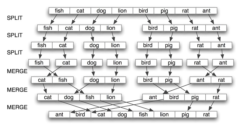
Figure 4.8: Sorting by Divide-and-Conquer: to sort an array, we split it in half and sort each half (recursively); we merge each sorted half back into a whole list (again recursively); this algorithm is known as "Merge Sort".
Another example is the process of looking up a word in a dictionary. We open the book somewhere around the middle and compare our word with the current page. If its earlier in the dictionary we repeat the process on the first half; if its later we use the second half. This search method is called binary search since it splits the problem in half at every step.
In another approach to algorithm design, we attack a problem by transforming it into an instance of a problem we already know how to solve. For example, in order to detect duplicate entries in a list, we can pre-sort the list, then scan through it once to check if any adjacent pairs of elements are identical.
Recursion 递归
The above examples of sorting and searching have a striking property: to solve a problem of size n, we have to break it in half and then work on one or more problems of size n/2. A common way to implement such methods uses recursion. We define a function f which simplifies the problem, and calls itself to solve one or more easier instances of the same problem. It then combines the results into a solution for the original problem.
For example, suppose we have a set of n words, and want to calculate how many different ways they can be combined to make a sequence of words. If we have only one word (n=1), there is just one way to make it into a sequence. If we have a set of two words, there are two ways to put them into a sequence. For three words there are six possibilities. In general, for n words, there are n × n-1 × … × 2 × 1 ways (i.e. the factorial of n). We can code this up as follows:
|
However, there is also a recursive algorithm for solving this problem, based on the following observation. Suppose we have a way to construct all orderings for n-1 distinct words. Then for each such ordering, there are n places where we can insert a new word: at the start, the end, or any of the n-2 boundaries between the words. Thus we simply multiply the number of solutions found for n-1 by the value of n. We also need the base case, to say that if we have a single word, there's just one ordering. We can code this up as follows:
|
These two algorithms solve the same problem. One uses iteration while the other uses recursion. We can use recursion to navigate a deeply-nested object, such as the WordNet hypernym hierarchy(我们可以使用递归来导航一个深度嵌套的对象,诸如WordNet上位词层次). Let's count the size of the hypernym hierarchy rooted at a given synset s. We'll do this by finding the size of each hyponym of s, then adding these together (we will also add 1 for the synset itself). The following function size1() does this work; notice that the body of the function includes a recursive call to size1():
|
We can also design an iterative solution to this problem which processes the hierarchy in layers. The first layer is the synset itself , then all the hyponyms of the synset, then all the hyponyms of the hyponyms. Each time through the loop it computes the next layer by finding the hyponyms of everything in the last layer . It also maintains a total of the number of synsets encountered so far .
|
Not only is the iterative solution much longer, it is harder to interpret. It forces us to think procedurally, and keep track of what is happening with the layer and total variables through time. Let's satisfy ourselves that both solutions give the same result. We'll use a new form of the import statement, allowing us to abbreviate the name wordnet to wn:
|
As a final example of recursion, let's use it to construct a deeply-nested object. A letter trie(字母Trie树) is a data structure that can be used for indexing a lexicon, one letter at a time. (The name is based on the word retrieval). For example, if trie contained a letter trie, then trie['c'] would be a smaller trie which held all words starting with c. Example 4.9 demonstrates the recursive process of building a trie, using Python dictionaries (Section 5.3). To insert the word chien (French for dog), we split off the c and recursively insert hien into the sub-trie trie['c']. The recursion continues until there are no letters remaining in the word, when we store the intended value (in this case, the word dog).
| ||
| ||
|
Example 4.9 (code_trie.py): Building a Letter Trie: A recursive function that builds a nested dictionary structure; each level of nesting contains all words with a given prefix, and a sub-trie containing all possible continuations. |
![]() Caution!
Caution!
Despite the simplicity of recursive programming, it comes with a cost. Each time a function is called, some state information needs to be pushed on a stack, so that once the function has completed, execution can continue from where it left off. For this reason, iterative solutions are often more efficient than recursive solutions.
尽管递归编程更简洁,然而它伴随着额外的代价。每次函数调用,一些状态信息需要推进栈中,所以一旦该函数完成,执行将从它离开的地方继续。因此,迭代解决常常比递归的效率更高。
Space-Time Tradeoffs 时空权衡
We can sometimes significantly speed up the execution of a program by building an auxiliary data structure(辅助数据结构), such as an index. The listing in Example 4.10 implements a simple text retrieval system for the Movie Reviews Corpus. By indexing the document collection it provides much faster lookup.
| ||
|
Example 4.10 (code_search_documents.py): A Simple Text Retrieval System |
A more subtle example of a space-time tradeoff involves replacing the tokens of a corpus with integer identifiers. We create a vocabulary for the corpus, a list in which each word is stored once, then invert this list so that we can look up any word to find its identifier. Each document is preprocessed, so that a list of words becomes a list of integers. Any language models can now work with integers. See the listing in Example 4.11 for an example of how to do this for a tagged corpus.
| ||
|
Example 4.11 (code_strings_to_ints.py): Preprocess tagged corpus data, converting all words and tags to integers |
Another example of a space-time tradeoff is maintaining a vocabulary list. If you need to process an input text to check that all words are in an existing vocabulary, the vocabulary should be stored as a set, not a list. The elements of a set are automatically indexed, so testing membership of a large set will be much faster than testing membership of the corresponding list.
We can test this claim using the timeit module. The Timer class has two parameters, a statement which is executed multiple times, and setup code that is executed once at the beginning. We will simulate a vocabulary of 100,000 items using a list or set of integers. The test statement will generate a random item which has a 50% chance of being in the vocabulary .(这样的写法还是第一次见,学习了...
Timer的使用说明
class timeit.Timer([stmt='pass'[, setup='pass'[, timer=<timer function>]]])
Class for timing execution speed of small code snippets.
The constructor takes a statement to be timed, an additional statement used for setup, and a timer function. Both statements default to 'pass'; the timer function is platform-dependent (see the module doc string). stmt and setup may also contain multiple statements separated by ; or newlines, as long as they don’t contain multi-line string literals.
To measure the execution time of the first statement, use the timeit() method. The repeat() method is a convenience to call timeit() multiple times and return a list of results.
Changed in version 2.6: The stmt and setup parameters can now also take objects that are callable without arguments. This will embed calls to them in a timer function that will then be executed by timeit(). Note that the timing overhead is a little larger in this case because of the extra function calls.
关于这个模块的详细说明在http://docs.python.org/library/timeit.html )
|
Performing 1000 list membership tests takes a total of 2.8 seconds, while the equivalent tests on a set take a mere 0.0037 seconds, or three orders of magnitude(数量级) faster!
Dynamic Programming 动态编程
Dynamic programming is a general technique for designing algorithms which is widely used in natural language processing. The term 'programming' is used in a different sense to what you might expect, to mean planning or scheduling. Dynamic programming is used when a problem contains overlapping sub-problems(动态编程被用于问题包含有重叠的子问题). Instead of computing solutions to these sub-problems repeatedly, we simply store them in a lookup table. In the remainder of this section we will introduce dynamic programming, but in a rather different context to syntactic parsing.
Pingala was an Indian author who lived around the 5th century B.C., and wrote a treatise(专著) on Sanskrit prosody(梵文韵律) called the Chandas Shastra. Virahanka extended this work around the 6th century A.D., studying the number of ways of combining short and long syllables to create a meter of length n. Short syllables, marked S, take up one unit of length, while long syllables(音节), marked L, take two. Pingala found, for example, that there are five ways to construct a meter of length 4: V4 = {LL, SSL, SLS, LSS, SSSS}. Observe that we can split V4 into two subsets, those starting with L and those starting with S, as shown in (1).
|
(1) |
|
V4 = LL, LSS i.e. L prefixed to each item of V2 = {L, SS} SSL, SLS, SSSS i.e. S prefixed to each item of V3 = {SL, LS, SSS} |
| ||
| ||
|
Example 4.12 (code_virahanka.py): Four Ways to Compute Sanskrit Meter: (i) iterative; (ii) bottom-up dynamic programming; (iii) top-down dynamic programming; and (iv) built-in memoization. |
With this observation, we can write a little recursive function called virahanka1() to compute these meters, shown in Example 4.12. Notice that, in order to compute V4 we first compute V3 and V2. But to compute V3, we need to first compute V2 and V1. This call structure(调用结构) is depicted in (2).
|
(2) |
|
|
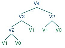
As you can see, V2 is computed twice. This might not seem like a significant problem, but it turns out to be rather wasteful as n gets large: to compute V20 using this recursive technique, we would compute V2 4,181 times; and for V40 we would compute V2 63,245,986 times! A much better alternative is to store the value of V2 in a table and look it up whenever we need it. (一个更好的代替方法是把V2的值存储到一个表中并且当我们需要的时候就去查询)The same goes for other values, such as V3 and so on. Function virahanka2() implements a dynamic programming approach to the problem. It works by filling up(填装) a table (called lookup) with solutions to all smaller instances of the problem, stopping as soon as we reach the value we're interested in. At this point we read off the value and return it. Crucially, each sub-problem is only ever solved once.
Notice that the approach taken in virahanka2() is to solve smaller problems on the way to solving larger problems(注意在该函数中所采用的这个方法是通过解决较小的问题来解决这些较大的问题). Accordingly, this is known as the bottom-up approach to dynamic programming.(因此,这个也被称为是动态编程的自底向上的方法) Unfortunately it turns out to be quite wasteful for some applications, since it may compute solutions to sub-problems that are never required for solving the main problem. This wasted computation can be avoided using the top-down approach to dynamic programming, which is illustrated in the functionvirahanka3() in Example 4.12. Unlike the bottom-up approach, this approach is recursive(这个自顶向下的方法是递归地). It avoids the huge wastage of virahanka1() by checking whether it has previously stored the result. If not, it computes the result recursively and stores it in the table. The last step is to return the stored result. The final method, invirahanka4(), is to use a Python "decorator" called memoize, which takes care of the housekeeping work done by virahanka3() without cluttering up(乱堆) the program. This "memoization" process stores the result of each previous call to the function along with the parameters that were used. (最后的这个方法invirahanka4(),使用了Python名为memoize的装饰器,包含了invirahanka3()所做的工作而没有打乱程序)If the function is subsequently called with the same parameters, it returns the stored result instead of recalculating it. (This aspect of Python syntax is beyond the scope of this book.)
This concludes our brief introduction to dynamic programming. We will encounter it again in Section 8.4.

 浙公网安备 33010602011771号