

1. 写在前面
最近在做边缘检测方面的一些工作,在网络上也找了很多有用的资料,感谢那些积极分享知识的先辈们,自己在理解Canny边缘检测算法的过程中也走了一些弯路,在编程实现的过程中,也遇到了一个让我怀疑人生的BUG(日了狗狗)。就此写下此文,作为后记,也希望此篇文章可以帮助那些在理解Canny算法的道路上暂入迷途的童鞋。废话少说,上干货。
2. Canny边缘检测算法的发展历史
Canny边缘检测于1986年由JOHN CANNY首次在论文《A Computational Approach to Edge Detection》中提出,就此拉开了Canny边缘检测算法的序幕。
Canny边缘检测是从不同视觉对象中提取有用的结构信息并大大减少要处理的数据量的一种技术,目前已广泛应用于各种计算机视觉系统。Canny发现,在不同视觉系统上对边缘检测的要求较为类似,因此,可以实现一种具有广泛应用意义的边缘检测技术。边缘检测的一般标准包括:
1) 以低的错误率检测边缘,也即意味着需要尽可能准确的捕获图像中尽可能多的边缘。
2) 检测到的边缘应精确定位在真实边缘的中心。
3) 图像中给定的边缘应只被标记一次,并且在可能的情况下,图像的噪声不应产生假的边缘。
为了满足这些要求,Canny使用了变分法。Canny检测器中的最优函数使用四个指数项的和来描述,它可以由高斯函数的一阶导数来近似。
在目前常用的边缘检测方法中,Canny边缘检测算法是具有严格定义的,可以提供良好可靠检测的方法之一。由于它具有满足边缘检测的三个标准和实现过程简单的优势,成为边缘检测最流行的算法之一。
3. Canny边缘检测算法的处理流程
Canny边缘检测算法可以分为以下5个步骤:
1) 使用高斯滤波器,以平滑图像,滤除噪声。
2) 计算图像中每个像素点的梯度强度和方向。
3) 应用非极大值(Non-Maximum Suppression)抑制,以消除边缘检测带来的杂散响应。
4) 应用双阈值(Double-Threshold)检测来确定真实的和潜在的边缘。
5) 通过抑制孤立的弱边缘最终完成边缘检测。
下面详细介绍每一步的实现思路。
3.1 高斯平滑滤波
为了尽可能减少噪声对边缘检测结果的影响,所以必须滤除噪声以防止由噪声引起的错误检测。为了平滑图像,使用高斯滤波器与图像进行卷积,该步骤将平滑图像,以减少边缘检测器上明显的噪声影响。大小为(2k+1)x(2k+1)的高斯滤波器核的生成方程式由下式给出:
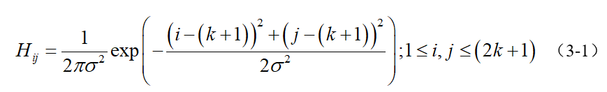
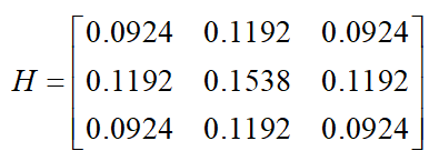
下面是一个sigma = 1.4,尺寸为3x3的高斯卷积核的例子(需要注意归一化):
若图像中一个3x3的窗口为A,要滤波的像素点为e,则经过高斯滤波之后,像素点e的亮度值为:

其中*为卷积符号,sum表示矩阵中所有元素相加求和。
重要的是需要理解,高斯卷积核大小的选择将影响Canny检测器的性能。尺寸越大,检测器对噪声的敏感度越低,但是边缘检测的定位误差也将略有增加。一般5x5是一个比较不错的trade off。
3.2 计算梯度强度和方向
图像中的边缘可以指向各个方向,因此Canny算法使用四个算子来检测图像中的水平、垂直和对角边缘。边缘检测的算子(如Roberts,Prewitt,Sobel等)返回水平Gx和垂直Gy方向的一阶导数值,由此便可以确定像素点的梯度G和方向theta 。

其中G为梯度强度, theta表示梯度方向,arctan为反正切函数。下面以Sobel算子为例讲述如何计算梯度强度和方向。
x和y方向的Sobel算子分别为:
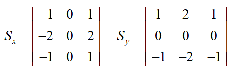
其中Sx表示x方向的Sobel算子,用于检测y方向的边缘; Sy表示y方向的Sobel算子,用于检测x方向的边缘(边缘方向和梯度方向垂直)。在直角坐标系中,Sobel算子的方向如下图所示。
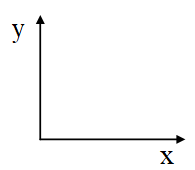
图3-1 Sobel算子的方向
若图像中一个3x3的窗口为A,要计算梯度的像素点为e,则和Sobel算子进行卷积之后,像素点e在x和y方向的梯度值分别为:

其中*为卷积符号,sum表示矩阵中所有元素相加求和。根据公式(3-2)便可以计算出像素点e的梯度和方向。
3.3 非极大值抑制
非极大值抑制是一种边缘稀疏技术,非极大值抑制的作用在于“瘦”边。对图像进行梯度计算后,仅仅基于梯度值提取的边缘仍然很模糊。对于标准3,对边缘有且应当只有一个准确的响应。而非极大值抑制则可以帮助将局部最大值之外的所有梯度值抑制为0,对梯度图像中每个像素进行非极大值抑制的算法是:
1) 将当前像素的梯度强度与沿正负梯度方向上的两个像素进行比较。
2) 如果当前像素的梯度强度与另外两个像素相比最大,则该像素点保留为边缘点,否则该像素点将被抑制。
通常为了更加精确的计算,在跨越梯度方向的两个相邻像素之间使用线性插值来得到要比较的像素梯度,现举例如下:
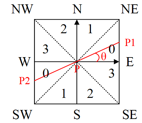
图3-2 梯度方向分割
如图3-2所示,将梯度分为8个方向,分别为E、NE、N、NW、W、SW、S、SE,其中0代表00~45o,1代表450~90o,2代表-900~-45o,3代表-450~0o。像素点P的梯度方向为theta,则像素点P1和P2的梯度线性插值为:
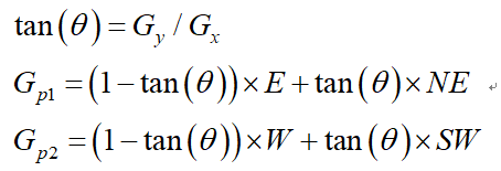
因此非极大值抑制的伪代码描写如下:
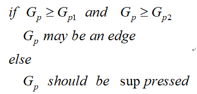
需要注意的是,如何标志方向并不重要,重要的是梯度方向的计算要和梯度算子的选取保持一致。
3.4 双阈值检测
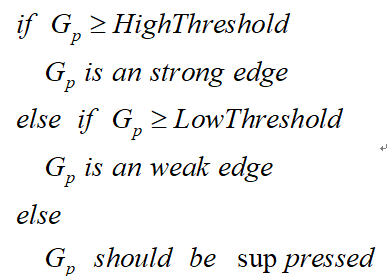
在施加非极大值抑制之后,剩余的像素可以更准确地表示图像中的实际边缘。然而,仍然存在由于噪声和颜色变化引起的一些边缘像素。为了解决这些杂散响应,必须用弱梯度值过滤边缘像素,并保留具有高梯度值的边缘像素,可以通过选择高低阈值来实现。如果边缘像素的梯度值高于高阈值,则将其标记为强边缘像素;如果边缘像素的梯度值小于高阈值并且大于低阈值,则将其标记为弱边缘像素;如果边缘像素的梯度值小于低阈值,则会被抑制。阈值的选择取决于给定输入图像的内容。
双阈值检测的伪代码描写如下:
3.5 抑制孤立低阈值点
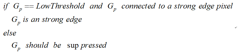
到目前为止,被划分为强边缘的像素点已经被确定为边缘,因为它们是从图像中的真实边缘中提取出来的。然而,对于弱边缘像素,将会有一些争论,因为这些像素可以从真实边缘提取也可以是因噪声或颜色变化引起的。为了获得准确的结果,应该抑制由后者引起的弱边缘。通常,由真实边缘引起的弱边缘像素将连接到强边缘像素,而噪声响应未连接。为了跟踪边缘连接,通过查看弱边缘像素及其8个邻域像素,只要其中一个为强边缘像素,则该弱边缘点就可以保留为真实的边缘。
抑制孤立边缘点的伪代码描述如下:
4 总结
通过以上5个步骤即可完成基于Canny算法的边缘提取,图5-1是该算法的检测效果图,希望对大家有所帮助。

图5-1 Canny边缘检测效果
附录是完整的MATLAB源码,可以直接拿来运行。
附录1
% -------------------------------------------------------------------------
%	Edge Detection Using Canny Algorithm.
%	Auther: Yongli Yan.
%	Mail: yanyongli@ime.ac.cn
%	Date: 2017.08.01.
%   The direction of Sobel operator.
%   ^(y)
%   |
%   |
%   |
%   0--------->(x)
%   Direction of Gradient:
%               3   2   1
%               0   P   0
%               1   2   3
%	P = Current Point.
%               NW  N  NE
%               W   P   E
%               SW  S  SE
%   Point Index:
%               f(x-1,y-1)		f(x-1,y)	f(x-1,y+1)
%               f(x,  y-1)		f(x,  y)	f(x,  y+1)
%               f(x+1,y-1)   	f(x+1,y)	f(x+1,y+1)
%   Parameters:
%   percentOfPixelsNotEdges: Used for selecting thresholds.
%   thresholdRatio: Low thresh is this fraction of the high.
% -------------------------------------------------------------------------
function imgCanny = edge_canny(I,gaussDim,sigma,percentOfPixelsNotEdges,thresholdRatio)
%% Gaussian smoothing filter.
m = gaussDim(1);
n = gaussDim(2);
if mod(m,2) == 0 || mod(n,2) == 0
    error('The dimensionality of Gaussian must be odd!');
end
% Generate gaussian convolution kernel.
gaussKernel = fspecial('gaussian', [m,n], sigma);
% Image edge copy.
[m,n] = size(gaussKernel);
[row,col,dim] = size(I);
if dim > 1
    imgGray = rgb2gray(I);
else
    imgGray = I;
end
imgCopy = imgReplicate(imgGray,(m-1)/2,(n-1)/2);
% Gaussian smoothing filter.
imgData = zeros(row,col);
for ii = 1:row
    for jj = 1:col
        window = imgCopy(ii:ii+m-1,jj:jj+n-1);
        GSF = window.*gaussKernel;
        imgData(ii,jj) = sum(GSF(:));
    end
end
%% Calculate the gradient values for each pixel.
% Sobel operator.
dgau2Dx = [-1 0 1;-2 0 2;-1 0 1];
dgau2Dy = [1 2 1;0 0 0;-1 -2 -1];
[m,n] = size(dgau2Dx);
% Image edge copy.
imgCopy = imgReplicate(imgData,(m-1)/2,(n-1)/2);
% To store the gradient and direction information.
gradx = zeros(row,col);
grady = zeros(row,col);
gradm = zeros(row,col);
dir = zeros(row,col); % Direction of gradient.
% Calculate the gradient values for each pixel.
for ii = 1:row
    for jj = 1:col
        window = imgCopy(ii:ii+m-1,jj:jj+n-1);
        dx = window.*dgau2Dx;
        dy = window.*dgau2Dy;
        dx = dx'; % Make the sum more accurate.
        dx = sum(dx(:));
        dy = sum(dy(:));
        gradx(ii,jj) = dx;
        grady(ii,jj) = dy;
        gradm(ii,jj) = sqrt(dx^2 + dy^2);
        % Calculate the angle of the gradient.
        theta = atand(dy/dx) + 90; % 0~180.
        % Determine the direction of the gradient.
        if (theta >= 0 && theta < 45)
            dir(ii,jj) = 2;
        elseif (theta >= 45 && theta < 90)
            dir(ii,jj) = 3;
        elseif (theta >= 90 && theta < 135)
            dir(ii,jj) = 0;
        else
            dir(ii,jj) = 1;
        end
    end
end
% Normalize for threshold selection.
magMax = max(gradm(:));
if magMax ~= 0
    gradm = gradm / magMax;
end
%% Plot 3D gradient graph.
% [xx, yy] = meshgrid(1:col, 1:row);
% figure;
% surf(xx,yy,gradm);
%% Threshold selection.
counts = imhist(gradm, 64);
highThresh = find(cumsum(counts) > percentOfPixelsNotEdges*row*col,1,'first') / 64;
lowThresh = thresholdRatio*highThresh;
%% Non-Maxima Suppression(NMS) Using Linear Interpolation.
gradmCopy = zeros(row,col);
imgBW = zeros(row,col);
for ii = 2:row-1
    for jj = 2:col-1
        E =  gradm(ii,jj+1);
        S =  gradm(ii+1,jj);
        W =  gradm(ii,jj-1);
        N =  gradm(ii-1,jj);
        NE = gradm(ii-1,jj+1);
        NW = gradm(ii-1,jj-1);
        SW = gradm(ii+1,jj-1);
        SE = gradm(ii+1,jj+1);
		% Linear interpolation.
        % dy/dx = tan(theta).
        % dx/dy = tan(90-theta).
		gradValue = gradm(ii,jj);
        if dir(ii,jj) == 0
            d = abs(grady(ii,jj)/gradx(ii,jj));
            gradm1 = E*(1-d) + NE*d;
            gradm2 = W*(1-d) + SW*d;
        elseif dir(ii,jj) == 1
            d = abs(gradx(ii,jj)/grady(ii,jj));
            gradm1 = N*(1-d) + NE*d;
            gradm2 = S*(1-d) + SW*d;
        elseif dir(ii,jj) == 2
            d = abs(gradx(ii,jj)/grady(ii,jj));
            gradm1 = N*(1-d) + NW*d;
            gradm2 = S*(1-d) + SE*d;
        elseif dir(ii,jj) == 3
            d = abs(grady(ii,jj)/gradx(ii,jj));
            gradm1 = W*(1-d) + NW*d;
            gradm2 = E*(1-d) + SE*d;
        else
            gradm1 = highThresh;
            gradm2 = highThresh;
        end
		% Non-Maxima Suppression.
        if gradValue >= gradm1 && gradValue >= gradm2
            if gradValue >= highThresh
                imgBW(ii,jj) = 1;
                gradmCopy(ii,jj) = highThresh;
            elseif gradValue >= lowThresh
                gradmCopy(ii,jj) = lowThresh;
            else
                gradmCopy(ii,jj) = 0;
            end
        else
            gradmCopy(ii,jj) = 0;
        end
    end
end
%% High-Low threshold detection.Double-Threshold.
% If the 8 pixels around the low threshold point have high threshold, then
% the low threshold pixel should be retained.
for ii = 2:row-1
    for jj = 2:col-1
        if gradmCopy(ii,jj) == lowThresh
            neighbors = [...
                gradmCopy(ii-1,jj-1),   gradmCopy(ii-1,jj), gradmCopy(ii-1,jj+1),...
                gradmCopy(ii,  jj-1),                       gradmCopy(ii,  jj+1),...
                gradmCopy(ii+1,jj-1),   gradmCopy(ii+1,jj), gradmCopy(ii+1,jj+1)...
                ];
            if ~isempty(find(neighbors) == highThresh)
                imgBW(ii,jj) = 1;
            end
        end
    end
end
imgCanny = logical(imgBW);
end
%% Local functions. Image Replicate.
function imgRep = imgReplicate(I,rExt,cExt)
[row,col] = size(I);
imgCopy = zeros(row+2*rExt,col+2*cExt);
% 4 edges and 4 corners pixels.
top = I(1,:);
bottom = I(row,:);
left = I(:,1);
right = I(:,col);
topLeftCorner = I(1,1);
topRightCorner = I(1,col);
bottomLeftCorner = I(row,1);
bottomRightCorner = I(row,col);
% The coordinates of the oroginal image after the expansion in the new graph.
topLeftR = rExt+1;
topLeftC = cExt+1;
bottomLeftR = topLeftR+row-1;
bottomLeftC = topLeftC;
topRightR = topLeftR;
topRightC = topLeftC+col-1;
bottomRightR = topLeftR+row-1;
bottomRightC = topLeftC+col-1;
% Copy original image and 4 edges.
imgCopy(topLeftR:bottomLeftR,topLeftC:topRightC) = I;
imgCopy(1:rExt,topLeftC:topRightC) = repmat(top,[rExt,1]);
imgCopy(bottomLeftR+1:end,bottomLeftC:bottomRightC) = repmat(bottom,[rExt,1]);
imgCopy(topLeftR:bottomLeftR,1:cExt) = repmat(left,[1,cExt]);
imgCopy(topRightR:bottomRightR,topRightC+1:end) = repmat(right,[1,cExt]);
% Copy 4 corners.
for ii = 1:rExt
    for jj = 1:cExt
        imgCopy(ii,jj) = topLeftCorner;
        imgCopy(ii,jj+topRightC) = topRightCorner;
        imgCopy(ii+bottomLeftR,jj) = bottomLeftCorner;
        imgCopy(ii+bottomRightR,jj+bottomRightC) = bottomRightCorner;
    end
end
imgRep = imgCopy;
end
%% End of file.
附录2
%% test file of canny algorithm.
close all;
clear all;
clc;
%%
img = imread('./picture/lena.jpg');
% img = imnoise(img,'salt & pepper',0.01);
%%
[~,~,dim] = size(img);
if dim > 1
    imgCanny1 = edge(rgb2gray(img),'canny'); % system function.
else
    imgCanny1 = edge(img,'canny'); % system function.
end
imgCanny2 = edge_canny(img,[5,5],1.4,0.9,0.4); % my function.
%%
figure;
subplot(2,2,1);
imshow(img);
title('original');
%%
subplot(2,2,3);
imshow(imgCanny1);
title('system function');
%%
subplot(2,2,4);
imshow(imgCanny2);
title('my function');
