
【Keras】从两个实际任务掌握图像分类
我们一般用深度学习做图片分类的入门教材都是MNIST或者CIFAR-10,因为数据都是别人准备好的,有的甚至是一个函数就把所有数据都load进来了,所以跑起来都很简单,但是跑完了,好像自己还没掌握图片分类的完整流程,因为他们没有经历数据处理的阶段,所以谈不上走过一遍深度学习的分类实现过程。今天我想给大家分享两个比较贴近实际的分类项目,从数据分析和处理说起,以Keras为工具,彻底掌握图像分类任务。
这两个分类项目就是:交通标志分类和票据分类。交通标志分类在无人驾驶或者与交通相关项目都有应用,而票据分类任务就更加贴切生活了,同时该项目也是我现在做的一个大项目中的子任务。这两个分类任务都是很贴近实际的练手好项目,希望经过这两个实际任务可以掌握好Keras这个工具,并且搭建一个用于图像分类的通用框架,以后做其他图像分类项目也可以得心应手。
先说配置环境:
- Python 3.5
- Keras==2.0.1,TesnsorFlow后端,CPU训练
一、交通标志分类
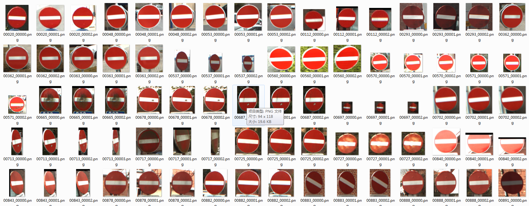
首先是观察数据,看看我们要识别的交通标志种类有多少,以及每一类的图片有多少。打开一看,这个交通标志的数据集已经帮我们分出了训练集和数据集。

每个文件夹的名字就是其标签。

每一类的标志图片数量在十来张到数十张,是一个小数据集,总的类别是62。


那我们开始以Keras为工具搭建一个图片分类器通用框架。
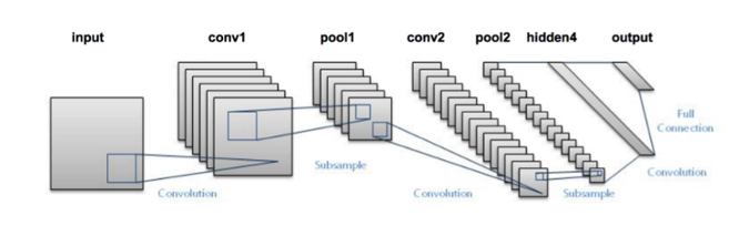
搭建CNN
用深度学习做图片分类选的网络肯定是卷积神经网络,但是现在CNN的种类这么多,哪一个会在我们这个标志分类任务表现最好?在实验之前,没有人会知道。一般而言,先选一个最简单又最经典的网络跑一下看看分类效果是的策略是明智的选择,那么LeNet肯定是最符合以上的要求啦,实现简单,又相当经典。那我们先单独写一个lenet.py的文件,然后实现改进版的LeNet类。
# import the necessary packages
from keras.models import Sequential
from keras.layers.convolutional import Conv2D
from keras.layers.convolutional import MaxPooling2D
from keras.layers.core import Activation
from keras.layers.core import Flatten
from keras.layers.core import Dense
from keras import backend as K

class LeNet:
    @staticmethod
    def build(width, height, depth, classes):
        # initialize the model
        model = Sequential()
        inputShape = (height, width, depth)
        # if we are using "channels last", update the input shape
        if K.image_data_format() == "channels_first":   #for tensorflow
            inputShape = (depth, height, width)
        # first set of CONV => RELU => POOL layers
        model.add(Conv2D(20, (5, 5),padding="same",input_shape=inputShape))
        model.add(Activation("relu"))
        model.add(MaxPooling2D(pool_size=(2, 2), strides=(2, 2)))
        #second set of CONV => RELU => POOL layers
        model.add(Conv2D(50, (5, 5), padding="same"))
        model.add(Activation("relu"))
        model.add(MaxPooling2D(pool_size=(2, 2), strides=(2, 2)))
        # first (and only) set of FC => RELU layers
        model.add(Flatten())
        model.add(Dense(500))
        model.add(Activation("relu"))

        # softmax classifier
        model.add(Dense(classes))
        model.add(Activation("softmax"))

        # return the constructed network architecture
        return model
其中conv2d表示执行卷积,maxpooling2d表示执行最大池化,Activation表示特定的激活函数类型,Flatten层用来将输入“压平”,用于卷积层到全连接层的过渡,Dense表示全连接层(500个神经元)。
参数解析器和一些参数的初始化
首先我们先定义好参数解析器。
# set the matplotlib backend so figures can be saved in the background
import matplotlib
matplotlib.use("Agg")

# import the necessary packages
from keras.preprocessing.image import ImageDataGenerator
from keras.optimizers import Adam
from sklearn.model_selection import train_test_split
from keras.preprocessing.image import img_to_array
from keras.utils import to_categorical
from imutils import paths
import matplotlib.pyplot as plt
import numpy as np
import argparse
import random
import cv2
import os
import sys
sys.path.append('..')
from net.lenet import LeNet


def args_parse():
    # construct the argument parse and parse the arguments
    ap = argparse.ArgumentParser()
    ap.add_argument("-dtest", "--dataset_test", required=True,
        help="path to input dataset_test")
    ap.add_argument("-dtrain", "--dataset_train", required=True,
        help="path to input dataset_train")
    ap.add_argument("-m", "--model", required=True,
        help="path to output model")
    ap.add_argument("-p", "--plot", type=str, default="plot.png",
        help="path to output accuracy/loss plot")
    args = vars(ap.parse_args())
    return args
我们还需要为训练设置一些参数,比如训练的epoches,batch_szie等。这些参数不是随便设的,比如batch_size的数值取决于你电脑内存的大小,内存越大,batch_size就可以设为大一点。又比如norm_size(图片归一化尺寸)是根据你得到的数据集,经过分析后得出的,因为我们这个数据集大多数图片的尺度都在这个范围内,所以我觉得32这个尺寸应该比较合适,但是不是最合适呢?那还是要通过实验才知道的,也许64的效果更好呢?
# initialize the number of epochs to train for, initial learning rate,
# and batch size
EPOCHS = 35
INIT_LR = 1e-3
BS = 32
CLASS_NUM = 62
norm_size = 32
载入数据
接下来我们需要读入图片和对应标签信息。
def load_data(path):
    print("[INFO] loading images...")
    data = []
    labels = []
    # grab the image paths and randomly shuffle them
    imagePaths = sorted(list(paths.list_images(path)))
    random.seed(42)
    random.shuffle(imagePaths)
    # loop over the input images
    for imagePath in imagePaths:
        # load the image, pre-process it, and store it in the data list
        image = cv2.imread(imagePath)
        image = cv2.resize(image, (norm_size, norm_size))
        image = img_to_array(image)
        data.append(image)

        # extract the class label from the image path and update the
        # labels list
        label = int(imagePath.split(os.path.sep)[-2])
        labels.append(label)

    # scale the raw pixel intensities to the range [0, 1]
    data = np.array(data, dtype="float") / 255.0
    labels = np.array(labels)

    # convert the labels from integers to vectors
    labels = to_categorical(labels, num_classes=CLASS_NUM)
    return data,labels
函数返回的是图片和其对应的标签。
训练
def train(aug,trainX,trainY,testX,testY,args):
    # initialize the model
    print("[INFO] compiling model...")
    model = LeNet.build(width=norm_size, height=norm_size, depth=3, classes=CLASS_NUM)
    opt = Adam(lr=INIT_LR, decay=INIT_LR / EPOCHS)
    model.compile(loss="categorical_crossentropy", optimizer=opt,
        metrics=["accuracy"])

    # train the network
    print("[INFO] training network...")
    H = model.fit_generator(aug.flow(trainX, trainY, batch_size=BS),
        validation_data=(testX, testY), steps_per_epoch=len(trainX) // BS,
        epochs=EPOCHS, verbose=1)

    # save the model to disk
    print("[INFO] serializing network...")
    model.save(args["model"])

    # plot the training loss and accuracy
    plt.style.use("ggplot")
    plt.figure()
    N = EPOCHS
    plt.plot(np.arange(0, N), H.history["loss"], label="train_loss")
    plt.plot(np.arange(0, N), H.history["val_loss"], label="val_loss")
    plt.plot(np.arange(0, N), H.history["acc"], label="train_acc")
    plt.plot(np.arange(0, N), H.history["val_acc"], label="val_acc")
    plt.title("Training Loss and Accuracy on traffic-sign classifier")
    plt.xlabel("Epoch #")
    plt.ylabel("Loss/Accuracy")
    plt.legend(loc="lower left")
    plt.savefig(args["plot"])
在这里我们使用了Adam优化器,由于这个任务是一个多分类问题,可以使用类别交叉熵(categorical_crossentropy)。但如果执行的分类任务仅有两类,那损失函数应更换为二进制交叉熵损失函数(binary cross-entropy)
主函数
#python train.py --dataset_train ../../traffic-sign/train --dataset_test ../../traffic-sign/test --model traffic_sign.model
if __name__=='__main__':
    args = args_parse()
    train_file_path = args["dataset_train"]
    test_file_path = args["dataset_test"]
    trainX,trainY = load_data(train_file_path)
    testX,testY = load_data(test_file_path)
    # construct the image generator for data augmentation
    aug = ImageDataGenerator(rotation_range=30, width_shift_range=0.1,
        height_shift_range=0.1, shear_range=0.2, zoom_range=0.2,
        horizontal_flip=True, fill_mode="nearest")
    train(aug,trainX,trainY,testX,testY,args)
在正式训练之前我们还使用了数据增广技术(ImageDataGenerator)来对我们的小数据集进行数据增强(对数据集图像进行随机旋转、移动、翻转、剪切等),以加强模型的泛化能力。
训练代码已经写好了,接下来开始训练(图片归一化尺寸为32,batch_size为32,epoches为35)。
python train.py --dataset_train ../../traffic-sign/train --dataset_test ../../traffic-sign/test --model traffic_sign.model
训练过程:
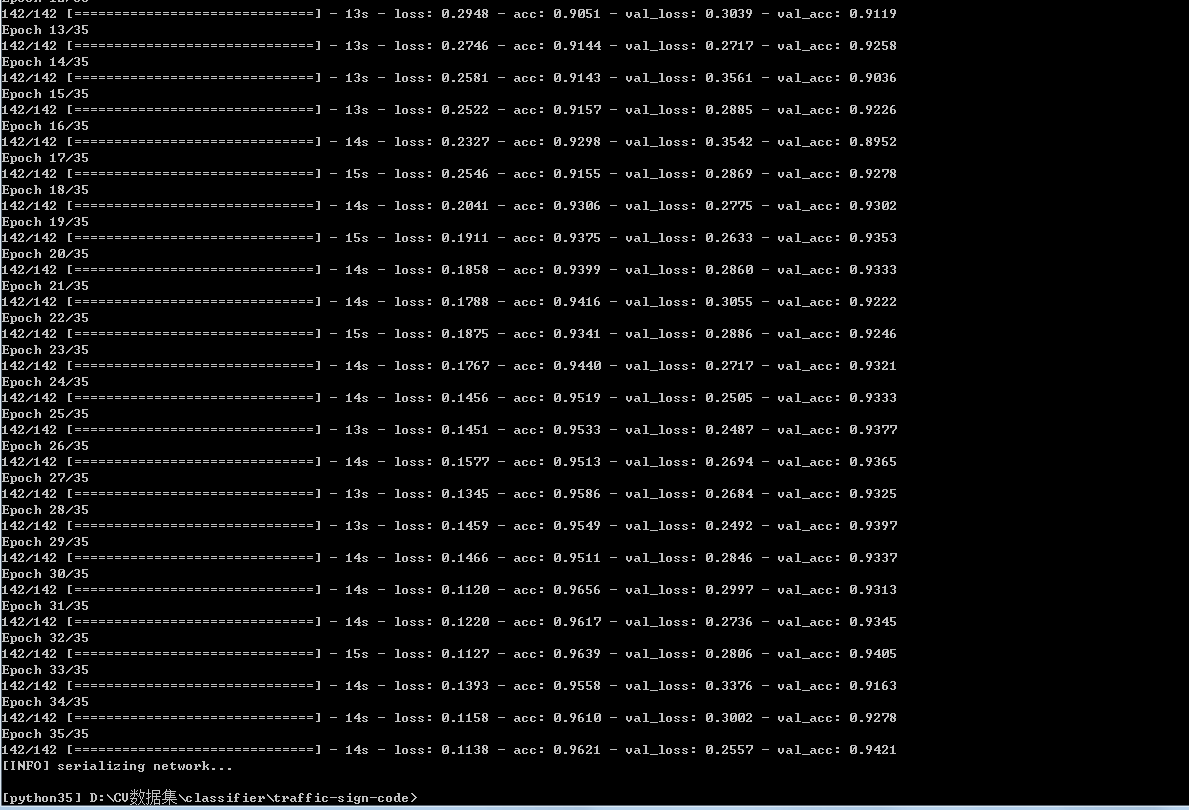
Loss和Accuracy:

从训练效果看来,准确率在94%左右,效果不错了。
预测单张图片
现在我们已经得到了我们训练好的模型traffic_sign.model,然后我们编写一个专门用于预测的脚本predict.py。
# import the necessary packages
from keras.preprocessing.image import img_to_array
from keras.models import load_model
import numpy as np
import argparse
import imutils
import cv2

norm_size = 32

def args_parse():
# construct the argument parse and parse the arguments
    ap = argparse.ArgumentParser()
    ap.add_argument("-m", "--model", required=True,
        help="path to trained model model")
    ap.add_argument("-i", "--image", required=True,
        help="path to input image")
    ap.add_argument("-s", "--show", action="store_true",
        help="show predict image",default=False)
    args = vars(ap.parse_args())
    return args


def predict(args):
    # load the trained convolutional neural network
    print("[INFO] loading network...")
    model = load_model(args["model"])

    #load the image
    image = cv2.imread(args["image"])
    orig = image.copy()

    # pre-process the image for classification
    image = cv2.resize(image, (norm_size, norm_size))
    image = image.astype("float") / 255.0
    image = img_to_array(image)
    image = np.expand_dims(image, axis=0)

    # classify the input image
    result = model.predict(image)[0]
    #print (result.shape)
    proba = np.max(result)
    label = str(np.where(result==proba)[0])
    label = "{}: {:.2f}%".format(label, proba * 100)
    print(label)

    if args['show']:
        # draw the label on the image
        output = imutils.resize(orig, width=400)
        cv2.putText(output, label, (10, 25),cv2.FONT_HERSHEY_SIMPLEX,
            0.7, (0, 255, 0), 2)
        # show the output image
        cv2.imshow("Output", output)
        cv2.waitKey(0)


#python predict.py --model traffic_sign.model -i ../2.png -s
if __name__ == '__main__':
    args = args_parse()
    predict(args)
预测脚本中的代码编写思路是:参数解析器-》载入训练好的模型-》读入图片信息-》预测-》展示预测效果。值得注意的是,参数-s是用于可视化结果的,加上他的话我们就可以看出我们输入的图片以及模型预测的分类结果,很直观。如果只需要得到分类结果,不加-s就可以了。
单张图片的预测:
python predict.py --model traffic_sign.model -i ../2.png -s
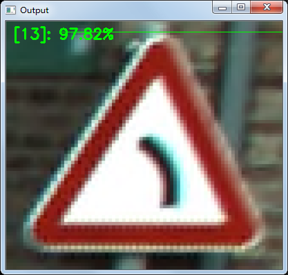
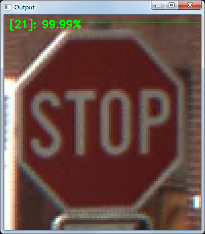
至此,交通分类任务完成。
这里分享一下这个项目的数据集来源:
你可以点击这里下载数据集。在下载页面上面有很多的数据集,但是你只需要下载 BelgiumTS for Classification (cropped images) 目录下面的两个文件:
- BelgiumTSC_Training (171.3MBytes)
- BelgiumTSC_Testing (76.5MBytes)
值得注意的是,原始数据集的图片格式是ppm,这是一种很老的图片保存格式,很多的工具都已经不支持它了。这也就意味着,我们不能很方便的查看这些文件夹里面的图片。
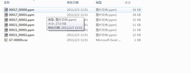
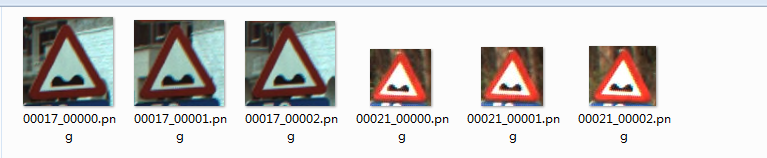
为了解决这个问题,我用opencv重新将这些图片转换为png格式,这样子我们就能很直观地看到数据图片了。
转换脚本在这里
同时我也把转换好的数据集传到百度云了,不想自己亲自转换的童鞋可以自行获取。
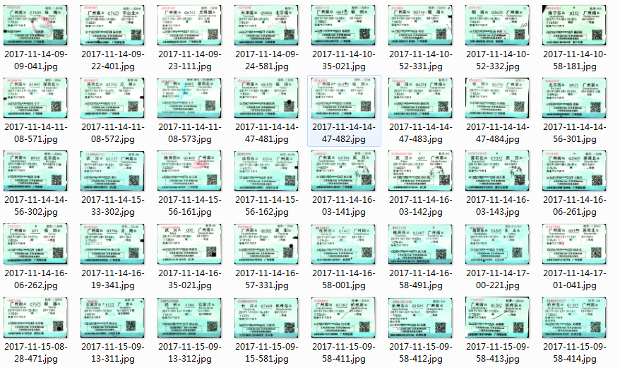
二、票据分类
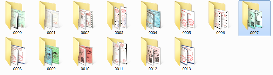
先分析任务和观察数据。我们这次的分类任务是票据分类,现在我们手头上的票据种类一共有14种,我们的任务就是训练一个模型将他们一一分类。先看看票据的图像吧。
票据种类一共14种,其图片名字就是其label。

票据是以下面所示的文件夹排布存储的。
然后我们再看一下每类图片数据的情况,看一下可利用的数据有多少。
有的票据数据比较少,也就十来张

有的票据比较多,有上百张
这样的数据分布直接拿去去训练的话,效果可能不会太好(这就是不平衡问题),但是这是后期模型调优时才需要考虑的问题,现在先放一边。那我们继续使用上面的图片分类框架完成本次的票据分类任务。
这次的数据集的存储方式与交通标志分类任务的数据存储不太一样,这个数据集没有把数据分成train和test两个文件夹,所以我们在代码中读取数据时写的函数应作出相应修改:我们先读取所有图片,再借助sklearn的“train_test_split”函数将数据集以一定比例分为训练集和测试集。
我写了个load_data2()函数来适应这种数据存储。
def load_data2(path):
    print("[INFO] loading images...")
    data = []
    labels = []
    # grab the image paths and randomly shuffle them
    imagePaths = sorted(list(paths.list_images(path)))
    random.seed(42)
    random.shuffle(imagePaths)
    # loop over the input images
    for imagePath in imagePaths:
        # load the image, pre-process it, and store it in the data list
        image = cv2.imread(imagePath)
        image = cv2.resize(image, (norm_size, norm_size))
        image = img_to_array(image)
        data.append(image)

        # extract the class label from the image path and update the
        # labels list
        label = int(imagePath.split(os.path.sep)[-2])
        labels.append(label)

    # scale the raw pixel intensities to the range [0, 1]
    data = np.array(data, dtype="float") / 255.0
    labels = np.array(labels)


    # partition the data into training and testing splits using 75% of
    # the data for training and the remaining 25% for testing
    (trainX, testX, trainY, testY) = train_test_split(data,
            labels, test_size=0.25, random_state=42)

    # convert the labels from integers to vectors
    trainY = to_categorical(trainY, num_classes=CLASS_NUM)
    testY = to_categorical(testY, num_classes=CLASS_NUM)
    return trainX,trainY,testX,testY
我们使用了sklearn中的神器train_test_split做了数据集的切分,非常方便。可以看出,load_data2()的返回值就是训练集图片和标注+测试集图片和标注。
在主函数也只需做些许修改就可以完成本次票据分类任务。
if __name__=='__main__':
    args = args_parse()
    file_path = args["dataset"]
    trainX,trainY,testX,testY = load_data2(file_path)
    # construct the image generator for data augmentation
    aug = ImageDataGenerator(rotation_range=30, width_shift_range=0.1,
        height_shift_range=0.1, shear_range=0.2, zoom_range=0.2,
        horizontal_flip=True, fill_mode="nearest")
    train(aug,trainX,trainY,testX,testY,args)
然后设定一些参数,比如图片归一化尺寸为64*64,训练35个epoches。设定完参数后我们开始训练。
python train.py --dataset ../../invoice_all/train --model invoice.model
训练的过程不算久,大概十来分钟。训练过程如下:

绘制出Loss和Accuracy曲线,可以看出,我们训练后的模型的准确率可以达到97%。直接使用一个LeNet网络就可以跑出这个准确率还是让人很开心的。

最后再用训练好的模型预测单张票据,看看效果:
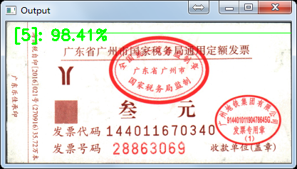
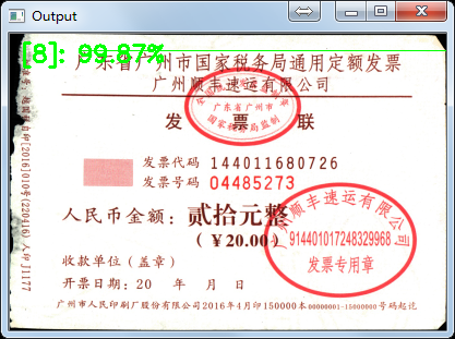
预测正确,deep learning 票据分类任务完成!
三、总结
我们使用了Keras搭建了一个基于LeNet的图片分类器的通用框架,并用它成功完成两个实际的分类任务。最后再说说我们现有的模型的一些改进的地方吧。第一,图片归一化的尺寸是否合适?比如票据分类任务中,图片归一化为64,可能这个尺寸有点小,如果把尺寸改为128或256,效果可能会更好;第二,可以考虑更深的网络,比如VGG,GoogLeNet等;第三,数据增强部分还可以再做一做。
完整代码和测试图片可以在我的github上获取。
参考资料:
https://www.pyimagesearch.com/2017/12/11/image-classification-with-keras-and-deep-learning/

