
机器学习实战——k-近邻算法
本章内容
================================
(一)什么是k-近邻分类算法
(二)怎样从文件中解析和导入数据
(三)使用Matplotlib创建扩散图
(四)对数据进行归一化
=================================
(一) 什么是k-近邻分类算法
简单地说,k-近邻算法采用测量不同特征值之间的距离方法进行分类,k-近邻是一种有监督的分类算法。
k-近邻的工作原理:存在一个样本数据集,也称之为训练样本集,并且样本集中的每个数据都存在标签,即每个样本所属的类别。输入没有标签的新数据,将新数据的每个特征与样本数据集中的每一个数据的特征进行比较,然后提取与新数据最相似的k个样本数据集,根据这k个样本数据集的类别标签,这k个样本数据中出现最多的类别即为新数据的类别标签。
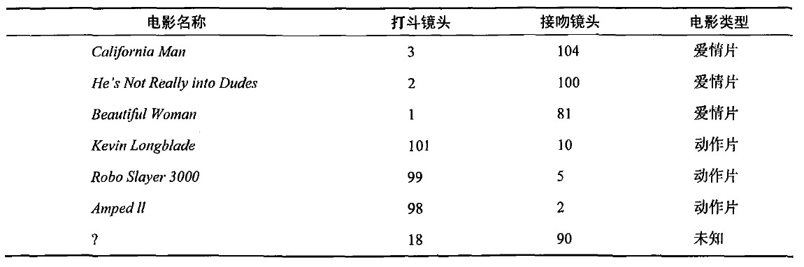
举例:根据表中提供的信息,求最后一部电影的电影类型?下图是每部电影的打斗镜头数、接吻镜头数以及电影评估类型
本文结合k-近邻分类算法的一般步骤,利用python代码实现。
k-近邻分类算法的一般步骤:
(1)导入数据
 1 from numpy import *
 2 import operator
 3
 4 def createDataSet():
 5     '''
 6     Use two arrays represent the information of chart.
 7     '''
 8     group = array([[3,104],[2,100],[1,81],[101,10],[99,5],[98,2]])
 9     label = ['love','love','love','action','action','action']
10     return group, label
(2)分类器的实现
 1 def classify(x, dataSet, label, k):
 2     '''
 3     The kNN classifier.
 4     '''
 5
 6     '''
 7     Compute the distance
 8     '''
 9     # shape return [m,n]
10     # m is the row number of the array
11     # n is the column number of the array
12     dataSetSize = dataSet.shape[0]
13     # tile can expand a vector to an array
14     # (dataSetSize, 1) expand row and column
15     # x = [1,3]
16     # print(tile(x,(3,1)))
17     # result [[1,3],[1,3],[1,3]]
18     diffMat = tile(x, (dataSetSize, 1)) - dataSet
19     sqDiffMat = diffMat ** 2
20     # sqDistance is a 1 x m array
21     sqDistance = sqDiffMat.sum(axis=1)
22     distances = sqDistance ** 0.5
23
24     '''
25     Choose the k samples, according to the distances
26     '''
27     sortedDistIndicies = distances.argsort()
28     classCount = {}
29     for i in range(k):
30         voteIlabel = label[sortedDistIndicies[i]]
31         classCount[voteIlabel] = classCount.get(voteIlabel, 0) + 1
32
33     '''
34     Sort and find the max class
35     '''
36     sortedClassCount = sorted(classCount.iteritems(),
37                               key = operator.itemgetter(1),
38                               reverse = True)
39     return sortedClassCount[0][0]
(3)测试新数据
group , labels = createDataSet()
x = [18, 90]
print(classify(x,group,labels,3))
(4)实验结果
1 love
===========================================
(二)怎样从文件中解析和导入数据
一般原始的数据存放在文本文件中,每个样本占据一行,N个样本就有N行.每个样本数据有n个特征,最后一列为样本的类别。
怎样将数据从文件中读取到数组中呢?
 1 def file2matrix(filename, n):
 2     f = open(filename)
 3     arrayOLines = f.readlines()
 4     numberOfLines = len(arrayOLines)
 5     returnMat = zeros((numberOfLines,n))
 6     classLabelVector = []
 7     index = 0
 8     for line in arrayOLines:
 9         line = line.strip()
10         listFormLine = line.split('\t')
11         returnMat[index,:] = listFormLine[0:n]
12         classLabelVector.append(int(listFormLine[-1]))
13         index += 1
14     return  returnMat, classLabelVector
==========================================
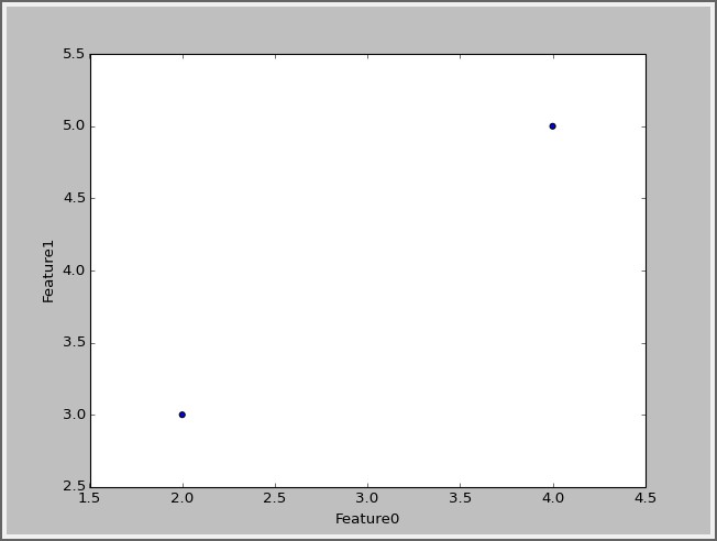
(三)使用Matplotlib创建散点图分析数据
Matplotlib可以将数据的两种类型的特征表示在一张2D的图中。
1 import matplotlib.pyplot as plt
2 from numpy import *
3 datmax = array([[2,3],[4,5]])
4 plt.scatter(datmax[:,0],datmax[:,1])
5 plt.xlabel('Feature0')
6 plt.ylabel('Feature1')
7 plt.show()
结果如下:
============================================
(四)归一化数值
如下图所示,我们很容易发现,使用欧式距离衡量数据之间的相似度,特数字差值最大的特征对计算结果影响最大,就如下图,每年获得的飞行常客里程数这个特征对计算结果的影响远大于其他两个特征的影响。若训练过程中,我们认为每一特征是等权重的。
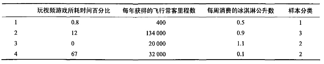
在处理这种不同取值范围的特征值时,我们通常采用的方法是将数值归一化,将取值范围处理为[0,1]或[-1,1]。
本文以最大最小进行归一化:
 1 from numpy import *
 2
 3 def autoNorm(dataSet):
 4     '''
 5     Use Max-min method to normalize the feature value
 6     '''
 7
 8     # find the min value of each feature
 9     # minVals is a 1 X m (m is the number of feature)
10     minVals = dataSet.min(0)
11     # find the max value of each feature
12     # maxVals is a 1 X m (m is the number of feature)
13     maxVals = dataSet.max(0)
14     ranges = maxVals - minVals
15     normDataSet = zeros(shape(dataSet))
16     # the number of samples
17     m = dataSet.shape[0]
18     normDataSet = dataSet - tile(minVals,(m,1))
19     normDataSet = normDataSet / tile(ranges,(m,1))
20     return normDataSet, minVals, ranges
测试数据:
10%作为测试集
90%作为训练集
 1 def datingClassTest():
 2     '''
 3     Test
 4     '''
 5     # hold out 10%
 6     hoRatio = 0.10
 7     # load dataSet file
 8     datingDataMat, datingLabels = file2matrix('datingTestSet2.txt')       #load data setfrom file
 9     normMat, ranges, minVals = autoNorm(datingDataMat)
10     m = normMat.shape[0]
11     numTestVecs = int(m*hoRatio)
12     errorCount = 0.0
13     for i in range(numTestVecs):
14         classifierResult = classify(normMat[i], normMat[numTestVecs:m], datingLabels[numTestVecs:m], 3)
15         if (classifierResult != datingLabels[i]):
16             errorCount += 1.0
17     print ("the total error rate is: %f" % (errorCount/float(numTestVecs)))
18     print errorCount,numTestVecs
===========================================
(五)总结
优点:精度高、对异常值不敏感、无数据输入假定。
缺点:计算复杂度高、空间复杂度高。
使用数据范围:数值型和标称型。

 浙公网安备 33010602011771号