
回归分析过程实例(练习)
By:HEHE
本实例是基于:混凝土抗压强度的回归分析
# 导包
import pandas as pd
import numpy as np
import matplotlib.pyplot as plt
plt.style.use('fivethirtyeight')
import seaborn as sns

%matplotlib inline

import warnings
warnings.filterwarnings('ignore')

import os
1. 数据基本面分析
# path
path_dir = os.path.dirname(os.path.dirname(os.getcwd()))

path_data = path_dir +  r'\concrete_data.xls'
# load_data
data = pd.read_excel(path_data)
# 查看数据基本面
data.head()
| Cement (component 1)(kg in a m^3 mixture) | Blast Furnace Slag (component 2)(kg in a m^3 mixture) | Fly Ash (component 3)(kg in a m^3 mixture) | Water (component 4)(kg in a m^3 mixture) | Superplasticizer (component 5)(kg in a m^3 mixture) | Coarse Aggregate (component 6)(kg in a m^3 mixture) | Fine Aggregate (component 7)(kg in a m^3 mixture) | Age (day) | Concrete compressive strength(MPa, megapascals) | |
|---|---|---|---|---|---|---|---|---|---|
| 0 | 540.0 | 0.0 | 0.0 | 162.0 | 2.5 | 1040.0 | 676.0 | 28 | 79.986111 |
| 1 | 540.0 | 0.0 | 0.0 | 162.0 | 2.5 | 1055.0 | 676.0 | 28 | 61.887366 |
| 2 | 332.5 | 142.5 | 0.0 | 228.0 | 0.0 | 932.0 | 594.0 | 270 | 40.269535 |
| 3 | 332.5 | 142.5 | 0.0 | 228.0 | 0.0 | 932.0 | 594.0 | 365 | 41.052780 |
| 4 | 198.6 | 132.4 | 0.0 | 192.0 | 0.0 | 978.4 | 825.5 | 360 | 44.296075 |
# 修改列名
data.columns = ['cement_component', 'furnace_slag', 'flay_ash', 'water_component', 'superplasticizer', \
    'coarse_aggregate', 'fine_aggregate', 'age', 'concrete_strength']
data.head()
| cement_component | furnace_slag | flay_ash | water_component | superplasticizer | coarse_aggregate | fine_aggregate | age | concrete_strength | |
|---|---|---|---|---|---|---|---|---|---|
| 0 | 540.0 | 0.0 | 0.0 | 162.0 | 2.5 | 1040.0 | 676.0 | 28 | 79.986111 |
| 1 | 540.0 | 0.0 | 0.0 | 162.0 | 2.5 | 1055.0 | 676.0 | 28 | 61.887366 |
| 2 | 332.5 | 142.5 | 0.0 | 228.0 | 0.0 | 932.0 | 594.0 | 270 | 40.269535 |
| 3 | 332.5 | 142.5 | 0.0 | 228.0 | 0.0 | 932.0 | 594.0 | 365 | 41.052780 |
| 4 | 198.6 | 132.4 | 0.0 | 192.0 | 0.0 | 978.4 | 825.5 | 360 | 44.296075 |
# 查看数据基本面
data.info()
<class 'pandas.core.frame.DataFrame'>
RangeIndex: 1030 entries, 0 to 1029
Data columns (total 9 columns):
cement_component     1030 non-null float64
furnace_slag         1030 non-null float64
flay_ash             1030 non-null float64
water_component      1030 non-null float64
superplasticizer     1030 non-null float64
coarse_aggregate     1030 non-null float64
fine_aggregate       1030 non-null float64
age                  1030 non-null int64
concrete_strength    1030 non-null float64
dtypes: float64(8), int64(1)
memory usage: 72.5 KB
# 查看数据基本面
data.describe()
| cement_component | furnace_slag | flay_ash | water_component | superplasticizer | coarse_aggregate | fine_aggregate | age | concrete_strength | |
|---|---|---|---|---|---|---|---|---|---|
| count | 1030.000000 | 1030.000000 | 1030.000000 | 1030.000000 | 1030.000000 | 1030.000000 | 1030.000000 | 1030.000000 | 1030.000000 |
| mean | 281.165631 | 73.895485 | 54.187136 | 181.566359 | 6.203112 | 972.918592 | 773.578883 | 45.662136 | 35.817836 |
| std | 104.507142 | 86.279104 | 63.996469 | 21.355567 | 5.973492 | 77.753818 | 80.175427 | 63.169912 | 16.705679 |
| min | 102.000000 | 0.000000 | 0.000000 | 121.750000 | 0.000000 | 801.000000 | 594.000000 | 1.000000 | 2.331808 |
| 25% | 192.375000 | 0.000000 | 0.000000 | 164.900000 | 0.000000 | 932.000000 | 730.950000 | 7.000000 | 23.707115 |
| 50% | 272.900000 | 22.000000 | 0.000000 | 185.000000 | 6.350000 | 968.000000 | 779.510000 | 28.000000 | 34.442774 |
| 75% | 350.000000 | 142.950000 | 118.270000 | 192.000000 | 10.160000 | 1029.400000 | 824.000000 | 56.000000 | 46.136287 |
| max | 540.000000 | 359.400000 | 200.100000 | 247.000000 | 32.200000 | 1145.000000 | 992.600000 | 365.000000 | 82.599225 |
数据基本面总结如下:
- 数据集共1030条数据,特征8个,目标为concrete_strength
- 数据集无缺失值,数据类型全为数值
2. EDA(数据探索性分析)
2.1 concrete_strength
sns.distplot(data['concrete_strength'], bins = 20, color = 'red')
<matplotlib.axes._subplots.AxesSubplot at 0x213da2c2080>
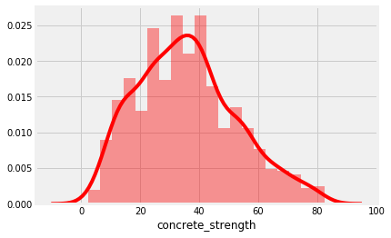
concrete_strength:数据分布正常,稍微有点右偏
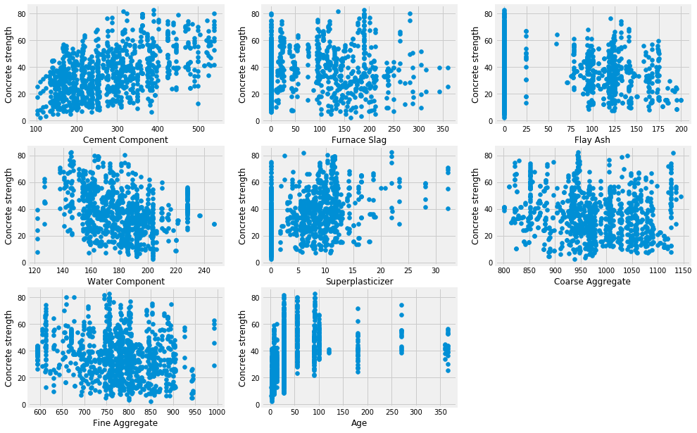
2.2 features
plt.figure(figsize = (15,10.5))
plot_count = 1

for feature in list(data.columns)[:-1]:
    plt.subplot(3,3, plot_count)
    plt.scatter(data[feature], data['concrete_strength'])
    plt.xlabel(feature.replace('_',' ').title())
    plt.ylabel('Concrete strength')
    plot_count +=1

plt.show()
plt.figure(figsize=(9,9))
corrmat = data.corr()
sns.heatmap(corrmat, vmax= 0.8, square = True, )
<matplotlib.axes._subplots.AxesSubplot at 0x213ddc4e7b8>
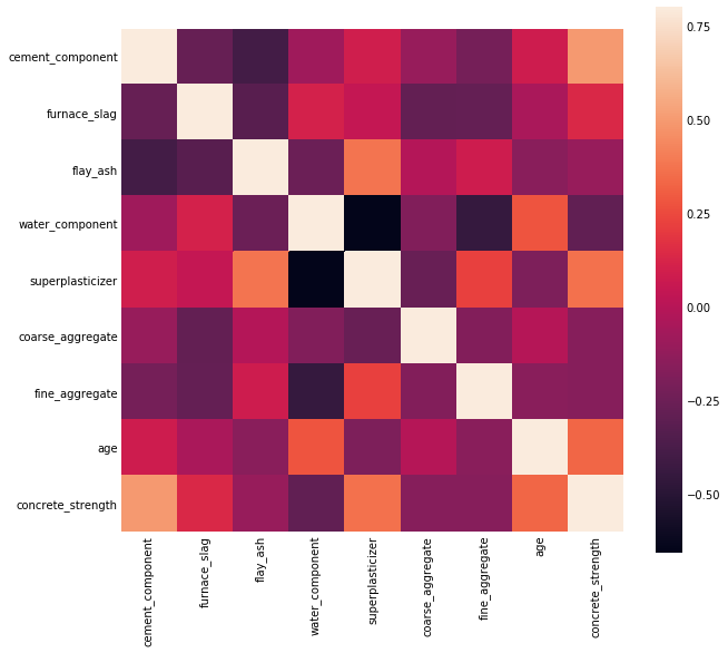
EDA总结:
- 数据相关性都不强,
- cement_component,water_component,superplasticizer,age似乎相关性高一点
- 由于特征都不多,可以分别用这四个特征以及所有特征尝试一遍
- 没有发现异常值
- 还没决定数据要不要标准化
3. model
实验内容:分别使用上面得到的特征,以及所有特征对混凝土强度做预测,同时使用不同的回归算法
from sklearn.model_selection import train_test_split
# 按数据集特征切割训练集测试集
def split_train_test(data, features=None, test_ratio=0.2):
    y = data['concrete_strength']
    if features != None:
        x = data[features]
    else:
        x = data.drop(['concrete_strength'], axis=1)
    train_x, test_x, train_y, test_y = train_test_split(x, y, test_size = test_ratio)
    return train_x, test_x, train_y, test_y
# 训练集,测试集
train_x, test_x, train_y, test_y = split_train_test(data, test_ratio = 0)
from sklearn.model_selection import GridSearchCV
from sklearn.model_selection import cross_val_score

from sklearn.linear_model import LinearRegression
from sklearn.linear_model import Ridge
from sklearn.linear_model import Lasso
from sklearn.linear_model import ElasticNet
from sklearn.ensemble import GradientBoostingRegressor
from sklearn.svm import SVR

from sklearn.metrics import r2_score
def data_cross_val(x,y, clfs, clfs_name, cv= 5):
    for i,clf in enumerate(clfs):
        scores = cross_val_score(estimator=clf, X= x, y= y, cv=cv, scoring ='r2')
        print(clfs_name[i])
        print('the R2 score: %f' %  np.mean(scores))
3.1 所有特征做回归
clfs = [LinearRegression(), Ridge(), Lasso(), ElasticNet(), GradientBoostingRegressor(), SVR()]
clfs_name = ['LinearRegression', 'Ridge', 'Lasso', 'ElasticNet', 'GradientBoostingRegressor', 'SVR']
data_cross_val(train_x, train_y, clfs,clfs_name, cv = 5)
LinearRegression
the R2 score: 0.604974
Ridge
the R2 score: 0.604974
Lasso
the R2 score: 0.605090
ElasticNet
the R2 score: 0.605220
GradientBoostingRegressor
the R2 score: 0.908837
SVR
the R2 score: 0.023249
结论:单一的回归器还是没有梯度提升机好,可以尝试用bagging和stacking的方式再实验一下,或者增加特征。
3.2 部分相关特征做回归
# 训练集,测试集
features = ['cement_component','water_component','superplasticizer','age']
train_x, test_x, train_y, test_y = split_train_test(data, features, test_ratio = 0)
clfs = [LinearRegression(), Ridge(), Lasso(), ElasticNet(), GradientBoostingRegressor(), SVR()]
clfs_name = ['LinearRegression', 'Ridge', 'Lasso', 'ElasticNet', 'GradientBoostingRegressor', 'SVR']
data_cross_val(train_x, train_y, clfs,clfs_name, cv = 5)
LinearRegression
the R2 score: 0.485046
Ridge
the R2 score: 0.485045
Lasso
the R2 score: 0.484828
ElasticNet
the R2 score: 0.484840
GradientBoostingRegressor
the R2 score: 0.830816
SVR
the R2 score: 0.043992
总结:目前来说使用部分相关的特征来做回归,由于特征数目太少,还不如用所有特征来的比较好
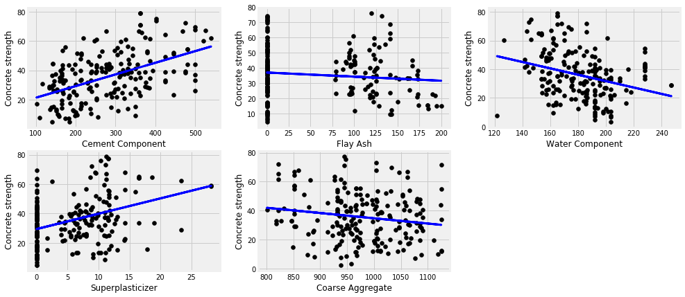
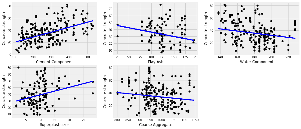
3.3 单线性回归
plt.figure(figsize=(15,7))
plot_count = 1

for feature in ['cement_component', 'flay_ash', 'water_component', 'superplasticizer', 'coarse_aggregate']:
    data_tr = data[['concrete_strength', feature]]

    x_train, x_test, y_train, y_test = split_train_test(data_tr, [feature])

    # Create linear regression object
    regr = LinearRegression()

    # Train the model using the training sets
    regr.fit(x_train, y_train)
    y_pred = regr.predict(x_test)

    # Plot outputs
    plt.subplot(2,3,plot_count)

    plt.scatter(x_test, y_test,  color='black')
    plt.plot(x_test, y_pred, color='blue',
             linewidth=3)
    plt.xlabel(feature.replace('_',' ').title())
    plt.ylabel('Concrete strength')

    print(feature, r2_score(y_test, y_pred))

    plot_count+=1

plt.show()
cement_component 0.24550132796330282
flay_ash 0.012228585601186226
water_component 0.09828887425075417
superplasticizer 0.11471267678235075
coarse_aggregate 0.02046823335033021
features = ['cement_component', 'flay_ash', 'water_component', 'superplasticizer', 'coarse_aggregate']

data_tr = data
data_tr=data_tr[(data_tr.T != 0).all()]

x_train, x_test, y_train, y_test = split_train_test(data_tr, features)

# Create linear regression object
regr = LinearRegression()

# Train the model using the training sets
regr.fit(x_train, y_train)
y_pred = regr.predict(x_test)

plt.scatter(range(len(y_test)), y_test,  color='black')
plt.plot(y_pred, color='blue', linewidth=3)

print('Features: %s'%str(features))
print('R2 score: %f'%r2_score(y_test, y_pred))
print('Intercept: %f'%regr.intercept_)
print('Coefficients: %s'%str(regr.coef_))
Features: ['cement_component', 'flay_ash', 'water_component', 'superplasticizer', 'coarse_aggregate']
R2 score: 0.155569
Intercept: 84.481913
Coefficients: [ 0.04304209 -0.02577486 -0.1747249   0.15980663 -0.02633656]

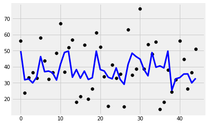
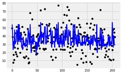
alphas = np.arange(0.1,5,0.1)

model = Ridge()
cv = GridSearchCV(estimator=model, param_grid=dict(alpha=alphas))

y_pred = cv.fit(x_train, y_train).predict(x_test)

plt.scatter(range(len(y_test)), y_test,  color='black')
plt.plot(y_pred, color='blue', linewidth=3)

print('Features: %s'%str(features))
print('R2 score: %f'%r2_score(y_test, y_pred))
print('Intercept: %f'%regr.intercept_)
print('Coefficients: %s'%str(regr.coef_))
Features: ['cement_component', 'flay_ash', 'water_component', 'superplasticizer', 'coarse_aggregate']
R2 score: 0.155562
Intercept: 84.481913
Coefficients: [ 0.04304209 -0.02577486 -0.1747249   0.15980663 -0.02633656]
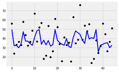
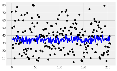
model = Lasso()
cv = GridSearchCV(estimator=model, param_grid=dict(alpha=alphas))

y_pred = cv.fit(x_train, y_train).predict(x_test)

plt.scatter(range(len(y_test)), y_test,  color='black')
plt.plot(y_pred, color='blue', linewidth=3)

print('Features: %s'%str(features))
print('R2 score: %f'%r2_score(y_test, y_pred))
print('Intercept: %f'%regr.intercept_)
print('Coefficients: %s'%str(regr.coef_))
Features: ['cement_component', 'flay_ash', 'water_component', 'superplasticizer', 'coarse_aggregate']
R2 score: 0.151682
Intercept: 84.481913
Coefficients: [ 0.04304209 -0.02577486 -0.1747249   0.15980663 -0.02633656]
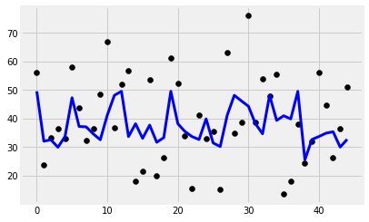
model = ElasticNet()
cv = GridSearchCV(estimator=model, param_grid=dict(alpha=alphas))

y_pred = cv.fit(x_train, y_train).predict(x_test)

plt.scatter(range(len(y_test)), y_test,  color='black')
plt.plot(y_pred, color='blue', linewidth=3)

print('Features: %s'%str(features))
print('R2 score: %f'%r2_score(y_test, y_pred))
print('Intercept: %f'%regr.intercept_)
print('Coefficients: %s'%str(regr.coef_))
Features: ['cement_component', 'flay_ash', 'water_component', 'superplasticizer', 'coarse_aggregate']
R2 score: 0.151796
Intercept: 84.481913
Coefficients: [ 0.04304209 -0.02577486 -0.1747249   0.15980663 -0.02633656]
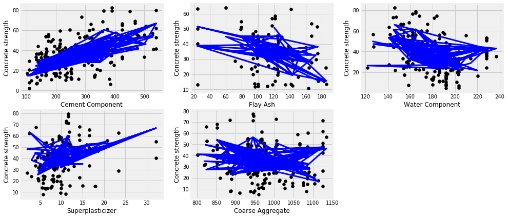
plt.figure(figsize=(15,7))
plot_count = 1

for feature in ['cement_component', 'flay_ash', 'water_component', 'superplasticizer', 'coarse_aggregate']:
    data_tr = data[['concrete_strength', feature]]
    data_tr=data_tr[(data_tr.T != 0).all()]

    x_train, x_test, y_train, y_test = split_train_test(data_tr, [feature])

    # Create linear regression object
    regr = GradientBoostingRegressor()

    # Train the model using the training sets
    regr.fit(x_train, y_train)
    y_pred = regr.predict(x_test)

    # Plot outputs
    plt.subplot(2,3,plot_count)

    plt.scatter(x_test, y_test,  color='black')
    plt.plot(x_test, y_pred, color='blue',
             linewidth=3)
    plt.xlabel(feature.replace('_',' ').title())
    plt.ylabel('Concrete strength')

    print(feature, r2_score(y_test, y_pred))

    plot_count+=1

plt.show()
cement_component 0.35248985320039705
flay_ash 0.17319875701989795
water_component 0.285023360910455
superplasticizer 0.19306275412216778
coarse_aggregate 0.17712532312647877
model = GradientBoostingRegressor()

y_pred = model.fit(x_train, y_train).predict(x_test)

plt.scatter(range(len(y_test)), y_test,  color='black')
plt.plot(y_pred, color='blue',
         linewidth=3)


print('Features: %s'%str(features))
print('R2 score: %f'%r2_score(y_test, y_pred))
#print('Intercept: %f'%regr.intercept_)
#print('Coefficients: %s'%str(regr.coef_))
Features: ['cement_component', 'flay_ash', 'water_component', 'superplasticizer', 'coarse_aggregate']
R2 score: 0.177125
plt.figure(figsize=(15,7))
plot_count = 1

for feature in ['cement_component', 'flay_ash', 'water_component', 'superplasticizer', 'coarse_aggregate']:
    data_tr = data[['concrete_strength', feature]]
    data_tr=data_tr[(data_tr.T != 0).all()]

    x_train, x_test, y_train, y_test = split_train_test(data_tr, [feature])

    # Create linear regression object
    regr = SVR(kernel='linear')

    # Train the model using the training sets
    regr.fit(x_train, y_train)
    y_pred = regr.predict(x_test)

    # Plot outputs
    plt.subplot(2,3,plot_count)

    plt.scatter(x_test, y_test,  color='black')
    plt.plot(x_test, y_pred, color='blue', linewidth=3)
    plt.xlabel(feature.replace('_',' ').title())
    plt.ylabel('Concrete strength')

    print(feature, r2_score(y_test, y_pred))

    plot_count+=1

plt.show()
cement_component 0.2054832593541437
flay_ash -0.044636249705873654
water_component 0.07749271320026574
superplasticizer 0.0671220299245393
coarse_aggregate 0.016036478490831563
model = SVR(kernel='linear')

y_pred = model.fit(x_train, y_train).predict(x_test)

plt.scatter(range(len(y_test)), y_test,  color='black')
plt.plot(y_pred, color='blue', linewidth=3)

print('Features: %s'%str(features))
print('R2 score: %f'%r2_score(y_test, y_pred))
Features: ['cement_component', 'flay_ash', 'water_component', 'superplasticizer', 'coarse_aggregate']
R2 score: 0.016036
4. 使用 cement_component和 water_component预测concrete_strength
feature = 'cement_component'
cc_new_data = np.array([[213.5]])

data_tr = data[['concrete_strength', feature]]
data_tr=data_tr[(data_tr.T != 0).all()]

x_train, x_test, y_train, y_test = split_train_test(data_tr, [feature])

regr = GradientBoostingRegressor()

# Train the model using the training sets

regr.fit(x_train, y_train)
cs_pred = regr.predict(cc_new_data)
print('Predicted value of concrete strength: %f'%cs_pred)
Predicted value of concrete strength: 36.472380
feature = 'water_component'
wc_new_data = np.array([[200]])

data_tr = data[['concrete_strength', feature]]
data_tr=data_tr[(data_tr.T != 0).all()]

x_train, x_test, y_train, y_test = split_train_test(data_tr, [feature])

regr = GradientBoostingRegressor()

# Train the model using the training sets
regr.fit(x_train, y_train)
cs_pred = regr.predict(wc_new_data)
print('Predicted value of concrete strength: %f'%cs_pred)
Predicted value of concrete strength: 32.648425

