
[Python] 05 - Load data from Files
Introduction
本篇比较实用,有必要仔细整理。
若干个相关的库:scipy,scikit-learning,pandas,matplotlib
读大数据文件
# 样例模板

beer_data = "recipeData.csv"

lines = (line for line in open(beer_data, encoding="ISO-8859-1"))
lists = (l.split(",") for l in lines)

#-----------------------------------------------------------------------------

# Take the column names out of the generator and store them, leaving only data
columns = next(lists)

# Take these columns and use them to create an informative dictionary
beerdicts = (dict(zip(columns, data)) for data in lists)
找合适的文件
filteredFiles = [f for f in listdir(dirPath) if isfile(join(dirPath, f)) and re.search(r'^[2]+',f)]
“文件读写” 的要点
一、文件打开
安全打开
二、文件读取
逐行读取
去杂质
三、二进制文件读取
mode='r'即可
txt到binary的互相转化
四、文件保存
pickle
json
"数据集文件”处理要点
一、CSV
Pandas Lib
二、Image
PIL Lib
"数据集划分" 的要点
常见数据集格式:.mat. npz, .data
train_test_split
文件读写
一、文件打开
传统方法的弊端
如果我们open一个文件之后,如果读写发生了异常,是不会调用close()的,那么这会造成文件描述符的资源浪费,久而久之,会造成系统的崩溃。
>>> f = open('data.txt', 'w')   # Make a new file in output mode ('w' is write)
>>> f.write('Hello\n')            # Write strings of characters to it
6
>>> f.write('world\n')            # Return number of items written in Python 3.X
6
>>> f.close()                     # Close to flush output buffers to disk
安全打开的建议
策略一:with...as...
with open(r'C:\code\data.txt') as myfile:     # See Chapter 34 for details
for line in myfile:
...use line here...
with方法,也叫"上下文管理器"。实现的样例如下:
可以看出,with ...as之后的语句,相当于调用了__enter__方法,在读取成功;或者异常它再调用__exit__方法。
class File():

    def __init__(self,filename,mode):
        self.filename = filename
        self.mode = mode

    def __enter__(self):
        print("entering")
        self.f = open(self.filename,self.mode)    # 读取失败则执行 __exit__
        return self.f

    def __exit__(self, exc_type, exc_val, exc_tb):
        print("will exit")


with File('out.txt','w') as f:
f.write("hello")
策略二:try...finally
myfile = open(r'C:\code\data.txt')
try:
  for line in myfile:
  ...use line here...
finally:
  myfile.close()
二、文件读取
一次性读完
>>> myfile = open('data.txt') # 'r' (read) is the default processing mode
>>> text = myfile.read() # Read entire file into a string

>>> text
'Hello\nworld\n'
>>> print(text) # print interprets control characters
Hello
world
>>> text.split() # File content is always a string
['Hello', 'world']
逐行读取
一行一行地读
file = open("sample.txt")
line = file.readline()            # 方案1.省内存
缓存效果逐行读
Ref: http://www.cnblogs.com/xuxn/archive/2011/07/27/read-a-file-with-python.html
带缓存的文件读取。[推荐:它每秒可以读96900行数据,效率是第一种方法的3倍]
# File: readline-example-3.py

file = open("sample.txt")

while 1:
lines = file.readlines(100000) # 方案2.通过预读,达到cache的效果
  if not lines:
      break
  for line in lines:
      pass # do something
yield处理大数据?
在python中 比如读取一个500G文件大小,如果使用readLines()方法和read()方法都是不可取的这样的话,直接会导致内存溢出,比较好的方法是使用read(limitSize)或 readLine(limitSize)方法读取数据,每次读取指定字节的数据,放置内存中。
更为直接的如下:python按行遍历一个大文件,最优的语法应该是什么?
with open('filename') as file:
    for line in file:
        do_things(line)

# 这是最快、最安全的方式
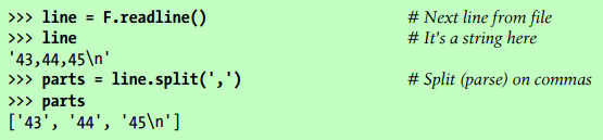
去杂质
(1) rstrip 去掉'\n'

(2) split 分割字符串
三、Binary Bytes Files
读取二进制
原数据是二进制
Python3默认就是utf8。如果用户不知道文件的格式的话可以不指定编码格式,同时直接使用rb的模式,直接以二进制的形式,就可以了。
f=open(file='D:/Users/tufengchao/Desktop/test123', mode='r',)
data=f.read()
print(data)
原数据非二进制
那么,就需要把二进制“解码”为“人眼可读”的形式。
>>> F = open('data.bin', 'rb')

>>> data = F.read()                            # Get packed binary data
>>> data
b'\x00\x00\x00\x07spam\x00\x08'

>>> import struct
>>> values = struct.unpack('>i4sh', data)      # Convert to Python objects
>>> values
(7, b'spam', 8)
保存二进制
原数据是二进制
直接write即可。
原数据非二进制
struct binary data: Storing Packed Binary Data
>>> F = open('data.bin', 'wb')                 # Open binary output file

>>> import struct
>>> data = struct.pack('>i4sh', 7, b'spam', 8) # Make packed binary data
>>> data
b'\x00\x00\x00\x07spam\x00\x08'

>>> F.write(data)                              # Write byte string
>>> F.close()
解释:
To create a packed binary data file, open it in 'wb' (write binary) mode, and pass struct a format string and some Python objects.
The format string used here means pack as a 4-byte integer, a 4-character string (which must be a bytes string as of Python 3.2), and a 2-byte integer,
all in big-endian form (other format codes handle padding bytes, floating-point numbers, and more):
More: 使用Python进行二进制文件读写的简单方法(推荐)
四、文件保存
如果是txt格式,则直接保持即可。
如果是其他格式 (PICKLE, JSON),则见机行事。
保存为 TXT
#1/list写入txt

ipTable = ['158.59.194.213', '18.9.14.13', '58.59.14.21']
fileObject = open('sampleList.txt', 'w')
for ip in ipTable:
    fileObject.write(ip)
    fileObject.write('\n')

fileObject.close()
保存为 Pickle
Pickle file: Storing Native Python Objects
[读]:pickle.load
[写]:pickle.dump
>>> D = {'a': 1, 'b': 2}
>>> F = open('datafile.pkl', 'wb')
--------------------------------------------------

>>> import pickle
>>> pickle.dump(D, F)      # 对象D存在文件里
>>> F.close()

>>> F = open('datafile.pkl', 'rb')
>>> E = pickle.load(F)     # 从文件中读出对象
>>> E
{'a': 1, 'b': 2}
保存为 Json
JSON file: Storing Python Objects
[读]:json.load
[写]:json.dump
>>> name = dict(first='Bob', last='Smith')            # 注意,变量就是Key
>>> rec  = dict(name=name, job=['dev', 'mgr'], age=40.5)
>>> rec
{'job': ['dev', 'mgr'], 'name': {'last': 'Smith', 'first': 'Bob'}, 'age': 40.5}
-------------------------------------------------------------------------------------

>>> import json
>>> json.dump(rec, fp=open('testjson.txt', 'w'), indent=4)
>>> print(open('testjson.txt').read())
{
  "job": [
    "dev",
    "mgr"
    ],
  "name": {
    "last": "Smith",
    "first": "Bob"
  },
  "age": 40.5
}

>>> P = json.load(open('testjson.txt'))
>>> P
{'job': ['dev', 'mgr'], 'name': {'last': 'Smith', 'first': 'Bob'}, 'age': 40.5}
数据集文件
数据分析常见的文件存储方式
- Python原生接口;
- Pandas也提供了方便的接口;
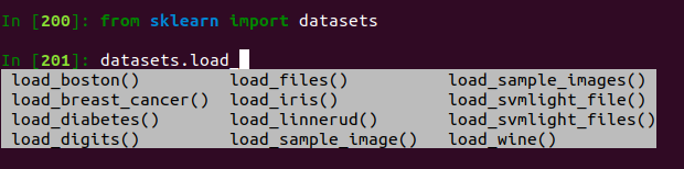
也可以直接读取默认内置数据集。
 make_biclusters()                make_classification()            make_gaussian_quantiles()        make_multilabel_classification() make_sparse_spd_matrix()
 make_blobs()                     make_friedman1()                 make_hastie_10_2()               make_regression()                make_sparse_uncorrelated()
 make_checkerboard()              make_friedman2()                 make_low_rank_matrix()           make_s_curve()                   make_spd_matrix()
 make_circles()                   make_friedman3()                 make_moons()                     make_sparse_coded_signal()       make_swiss_roll()
Ref: https://blog.csdn.net/wangdong2017/article/details/81326341
X1,Y1 = make_classification(n_samples=1000,n_features=2,n_redundant=0,n_informative=1,n_clusters_per_class=1)

X2,Y2 = make_classification(n_samples=1000,n_features=2,n_redundant=0,n_informative=2)

X2,Y2 = make_classification(n_samples=1000,n_features=2,n_redundant=0,n_informative=2)

X1,Y1 = make_classification(n_samples=1000,n_features=2,n_redundant=0,n_informative=2,n_clusters_per_class=1,n_classes=3)
# 1000个样本,2个属性,3种类别,方差分别为1.0,3.0,2.0
X1,Y1 = make_blobs(n_samples=1000,n_features=2,centers=3,cluster_std=[1.0,3.0,2.0])
plt.scatter(X1[:,0],X1[:,1],marker='o',c=Y1)
# make_gaussian_quantiles函数利用高斯分位点区分不同数据
X1,Y1 = make_gaussian_quantiles(n_samples=1000,n_features=2,n_classes=4)# make_hastie_10_2函数利用Hastie算法,生成2分类数据
X1,Y1 = make_hastie_10_2(n_samples=1000)   #

x1,y1 = make_circles(n_samples=1000,factor=0.5,noise=0.1)

x1,y1 = make_moons(n_samples=1000,noise=0.1)

一、CSV文件
“原生” 读 CSV文件
不考虑第一行 title
csv.reader():完全当成矩阵数据去读,省空间。
#!/usr/bin/python3
# -*- coding:utf-8 -*-
__author__ = 'mayi'

import csv

with open("test.csv", "r", encoding = "utf-8") as f:
    reader = csv.reader(f)

  rows   = [row    for row in reader]       # 打印出所有,如下
  column = [row[1] for row in reader]       # 打印一列
print(rows)

------------------------------------------------------------
结果:
[['No.', 'Name', 'Age', 'Score'],
 ['1', 'mayi', '18', '99'],
 ['2', 'jack', '21', '89'],
 ['3', 'tom', '25', '95'],
 ['4', 'rain', '19', '80']]
考虑第一行 作为Key值
csv.DictReader():
__author__ = 'mayi'

import csv

#读
with open("test.csv", "r", encoding = "utf-8") as f:
    reader = csv.DictReader(f)
    column = [row for row in reader]

print(column)
得到了不一样的结果,有点太细节了,哈哈。
[{'No.': '1', 'Age': '18', 'Score': '99', 'Name': 'mayi'},
 {'No.': '2', 'Age': '21', 'Score': '89', 'Name': 'jack'},
 {'No.': '3', 'Age': '25', 'Score': '95', 'Name': 'tom'},
 {'No.': '4', 'Age': '19', 'Score': '80', 'Name': 'rain'}]
“原生” 写 CSV文件
__author__ = 'mayi'

import csv

#写:追加
row = ['5', 'hanmeimei', '23', '81']

out = open("test.csv", "a", newline = "")

csv_writer = csv.writer(out, dialect = "excel")
csv_writer.writerow(row)
“pandas” 读 CSV文件
直接转化为二维数组的形式去处理。
有点类似数据库的 select 操作:goto [MySQL] 01- Basic sql
import pandas as pd

str_path = './data_analyst_sample_data.csv'
cols     = ['week_sold', 'price', 'num_sold', 'store_id', 'product_code', 'department_name']

dataset  = pd.read_csv(str_path, header=None, sep=',', names=cols)  # <---- 这里指定了 ”title"
-----------------------------------------------------------------------------------------------
total_price = 0.0
for i in range(1, len(dataset)):
    if (dataset['department_name'][i] == 'BEVERAGE'):
        each_price   = float(dataset['price'][i]) * float(dataset['num_sold'][i])
        each_price   = round(each_price, 2)
        total_price += each_price

print("Total price is %.2f" % total_price)
print("")
“pandas” 写 CSV文件
将DataFrame中的表格转化为csv文件。
import pandas as pd

raw_data = {'first_name': ['Jason', 'Molly', 'Tina', 'Jake', 'Amy'],
        'last_name': ['Miller', 'Jacobson', 'Ali', 'Milner', 'Cooze'],
        'age': [42, 52, 36, 24, 73],
        'preTestScore': [4, 24, 31, 2, 3],
        'postTestScore': [25, 94, 57, 62, 70]}
df = pd.DataFrame(raw_data, columns = ['first_name', 'last_name', 'age', 'preTestScore', 'postTestScore'])
df
df.to_csv("test.csv", index=False, sep='')
Output:
| first_name | last_name | age | preTestScore | postTestScore | |
|---|---|---|---|---|---|
| 0 | Jason | Miller | 42 | 4 | 25 |
| 1 | Molly | Jacobson | 52 | 24 | 94 |
| 2 | Tina | Ali | 36 | 31 | 57 |
| 3 | Jake | Milner | 24 | 2 | 62 |
| 4 | Amy | Cooze | 73 | 3 | 70 |
二、图片文件
Ref: https://www.jb51.net/article/102981.htm
"matplotlib + scipy" 操作并处理
读图:二维数组形式
使用了三个module干三件事情。
import matplotlib.pyplot as plt               # (a) plt 用于显示图片
import matplotlib.image  as mpimg             # (b) mpimg 用于读取图片
import numpy as np                            # (c) np用于处理图片
-------------------------------------------------------------------


lena = mpimg.imread('lena.png')          # 读取和代码处于同一目录下的 lena.png, however,0-1的值,需要自己乘以255

# 此时 lena 就已经是一个 np.array 了,可以对它进行任意处理
lena.shape #(512, 512, 3)

plt.imshow(lena)     # 显示图片
plt.axis('off')      # 不显示坐标轴
plt.show()
显示某个通道
利用 np.array 的性质,导出一个channel,再用 matplotlib 显示即可。
# 显示图片的第一个通道
lena_1 = lena[:,:,0]
plt.imshow('lena_1')
plt.show()

# 此时会发现显示的是热量图,不是我们预想的灰度图,可以添加 cmap 参数,有如下几种添加方法:
plt.imshow('lena_1', cmap='Greys_r')
plt.show()

img = plt.imshow('lena_1')
img.set_cmap('gray') # 'hot' 是热量图
plt.show()
将 RGB 转为灰度图
利用 np.array 的性质,需要靠自己使用 “点积” 来获得。
def rgb2gray(rgb):
  return np.dot(rgb[...,:3], [0.299, 0.587, 0.114])

gray =rgb2gray(lena)

# 也可以用 plt.imshow(gray, cmap = plt.get_cmap('gray'))
plt.imshow(gray, cmap='Greys_r')
plt.axis('off')
plt.show()
对图像进行放缩
Scikit-learning: Built on NumPy, SciPy, and matplotlib.
利用 scipy 的模块,进行缩放这样的高级操作。
from scipy import misc

lena_new_sz = misc.imresize(lena, 0.5) # 第二个参数如果是整数,则为百分比,如果是tuple,则为输出图像的尺寸

plt.imshow(lena_new_sz)
plt.axis('off')
plt.show()
保存图像
这里介绍了三种方法:
(a) plt保存:既然能显示,自然也能保存。
(b) scipy保存:既然是高级库,自然也能保存。
(c) np保存:既然在内存能保存图片,自然也能保存在硬盘里。
# 5.1 保存 matplotlib 画出的图像
该方法适用于保存任何 matplotlib 画出的图像,相当于一个 screencapture。

plt.imshow(lena_new_sz)
plt.axis('off')
plt.savefig('lena_new_sz.png')

-------------------------------------------------------------------------

# 5.2 将 array 保存为图像

from scipy import misc
misc.imsave('lena_new_sz.png', lena_new_sz)

-------------------------------------------------------------------------

5.3 直接保存 array
读取之后还是可以按照前面显示数组的方法对图像进行显示,这种方法完全不会对图像质量造成损失

np.save('lena_new_sz', lena_new_sz)        # 会在保存的名字后面自动加上.npy
img = np.load('lena_new_sz.npy')           # 读取前面保存的数组
“PIL” 图像处理标准库
PIL是Python平台事实上的图像处理标准库,支持多种格式,并提供强大的图形与图像处理功能。
打开、保存 图片
from PIL import Image

I = Image.open('lena.png')
I.save('new_lena.png')
显示 图片
from PIL import Image

im = Image.open('lena.png')
im.show()
PIL Image <----> np.array
也可以用 np.asarray(im) 区别是
(a) np.array() 是 "深拷贝"
(b) np.asarray() 是 "浅拷贝"
im_array = np.array(im) # 变换为数组,方便进一步处理
处理完毕后,还是要转换回PIL Image格式。
import matplotlib.image as mpimg
from PIL import Image

lena = mpimg.imread('lena.png')              # 这里读入的数据是 float32 型的,范围是0-1
im   = Image.fromarray(np.uinit8(lena*255))   # (1) 先变为np.array; (2) 然后再通过 fromarray() 变回 PIL Image
im.show()
RGB 转换为灰度图
from PIL import Image

I = Image.open('lena.png')
I.show()
L = I.convert('L')
L.show()
数据集划分
主要用于机器学习的数据集准备阶段。
数据 .npz 格式
读取数据
数据集本身已分为 train & test.
data = np.load('webkb.npz',)    #文档数据集

# training data
xtrain = data['xtrain']
ytrain = data['ytrain']

# test data
xtest = data['xtest']
ytest = data['ytest']

# which class is which?
class_label_strings = data['class_label_strings']

# we don't need the original any more
del(data)
数据 .mat 格式
读取数据
数据集本身已分为 train & test,但两者维度不同。
data = loadmat('./usps_gmm_3d.mat')  #手写字体数据集

xtrain3d = data['xtrain3d']
ytrain   = data['ytrain']

xtest3d = data['xtest3d']
ytest   = data['ytest']

pca_mu = data['mu']
pca_e  = data['E']
data.keys()
del(data)
另一个train 与 test 分开读取的例子。
import scipy.io as scio

train_file = '../data/trajectories_train.mat'
test_file  = '../data/trajectories_xtest.mat'
train_data = scio.loadmat(train_file)
test_data  = scio.loadmat(test_file)

x_train    = train_data['xtrain'][0]
y_train    = train_data['ytrain'][0]
key_train  = train_data['key'][0]
数据 .data 格式
读取数据
聚类数据,不用划分。实际上该数据就是csv格式。
with open('faithful.dat') as handle:
    # The first 25 lines are text, which we print out but don't use
    for i in range(25):
        print(handle.readline(), end="")
    #  The next part of the file we read using `pandas`
    data = pd.read_csv(handle, delim_whitespace=True)
查看基本信息
data.head(20)      #看前20个row的数据.

data.describe()    #查看统计信息
| eruptions | waiting | |
|---|---|---|
| count | 272.000000 | 272.000000 |
| mean | 3.487783 | 70.897059 |
| std | 1.141371 | 13.594974 |
| min | 1.600000 | 43.000000 |
| 25% | 2.162750 | 58.000000 |
| 50% | 4.000000 | 76.000000 |
| 75% | 4.454250 | 82.000000 |
| max | 5.100000 | 96.000000 |
手动划分数据集
原始数据
>>> import numpy as np
>>> from sklearn.model_selection import train_test_split

>>> X, y = np.arange(10).reshape((5, 2)), range(5)
>>> X
array([[0, 1],
       [2, 3],
       [4, 5],
       [6, 7],
       [8, 9]])

>>> list(y)
[0, 1, 2, 3, 4]
划分数据
>>> X_train, X_test, y_train, y_test = train_test_split( X, y, test_size=0.33, random_state=42 )

>>> X_train
array([[4, 5],
       [0, 1],
       [6, 7]])

>>> y_train
[2, 0, 3]

>>> X_test
array([[2, 3],
       [8, 9]])

>>> y_test
[1, 4]
End.

 浙公网安备 33010602011771号