[Scikit-learn] 1.5 Generalized Linear Models - SGD for Classification

NB：因为softmax，NN看上去是分类，其实是拟合（回归），拟合最大似然。

多分类参见：[Scikit-learn] 1.1 Generalized Linear Models - Logistic regression & Softmax

感知机采用的是形式最简单的梯度

Perceptron and SGDClassifier share the same underlying implementation.In fact, Perceptron() is equivalent to SGDClassifier(loss=”perceptron”, eta0=1, learning_rate=”constant”, penalty=None).

1.5. Stochastic Gradient Descent

损失函数

需要一些背景知识，参见斯坦福 CS231n - CNN for Visual Recognition 2 - lecture3

参考：斯坦福CS231n - CNN for Visual Recognition 2 - lecture3 Optimization

一、Loss function 计算

Linear SVM classifier的一个例子。

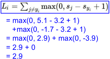
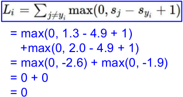
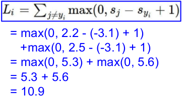
(1) 计算损失函数：Multiclass SVM loss

一个批次，三张图片，分别得到如下的预测值；而后计算loss。

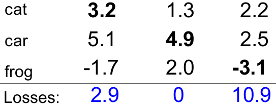
与"另外两个"的比较：

L = (2.9 + 0 + 10.9)/3
= 4.6

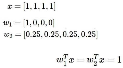
(2) 正则化

典型例子说服你：我们当然prefer后一个，w₂。

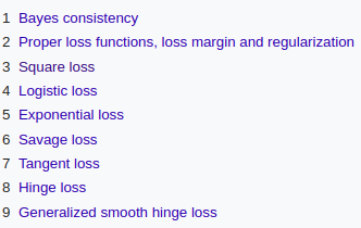
二、其他loss function

Ref: Loss functions for classification

三、loss计算对比

(a) Softmax classifier 的 Softmax's Loss 计算：

(b) Linear SVM classifier 的 hinge loss 计算：

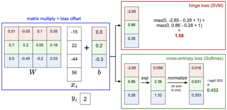
通过该演示体会：http://vision.stanford.edu/teaching/cs231n-demos/linear-classify/

梯度下降

一、逻辑回归

两种损失函数

第一步，逻辑回归的损失函数可以是“得分差”，当然也可以是其他。

第二步，利用“得分差”来进行梯度下降，进行参数优化。

常见有选择两种损失函数，如下：

（１）最小二乘损失函数：逻辑回归与梯度下降法全部详细推导

（２）交叉熵损失函数：机器学习算法 --- 逻辑回归及梯度下降（正统策略）

两个函数接口

Softmax参见：[Scikit-learn] 1.1 Generalized Linear Models - Logistic regression & Softmax

LogisticRegression (交叉熵损失，迭代) versus SGDClassifier(loss="log")

the major difference is the optimization algorithm:

Question: Liblinear/Coordinate Descent vs. Stochastic Gradient Descent.

问题：线性梯度下降　vs　随机梯度下降

If your problem is high dimensional (10K or more) and you have a large
number of examples (100K or more) you should choose the latter -
otherwise, LogisticRegression should be fine.

高维，更高的数据：随机梯度下降

反之：Liblinear/Coordinate梯度下降

迭代即可，
Both are not proper multinomial logistic regression models;

LogisticRegression does not care and simply computes the probability
estimates of each OVR classifier and normalized to make sure they sum
to one. You could do the same for SGDClassifier(loss='log') but you
have to implement it on your own. You should be aware of the fact that
SGDClassifier(n_jobs > 1) uses multiple processes, thus, if your
dataset (``X``) is too large (more than 50% of your RAM) you'll run
into troubles.

二、梯度下降实践

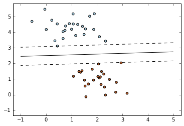
SGD + Linear SVM classifier

=========================================
SGD: Maximum margin separating hyperplane
=========================================

Plot the maximum margin separating hyperplane within a two-class
separable dataset using a linear Support Vector Machines classifier
trained using SGD.
"""
print(__doc__)

import numpy as np
import matplotlib.pyplot as plt
from sklearn.linear_model import SGDClassifier
from sklearn.datasets.samples_generator import make_blobs

# we create 50 separable points
X, Y = make_blobs(n_samples=50, centers=2, random_state=0, cluster_std=0.60)

# 生成样本（上），即刻训练（下）

# fit the model
clf = SGDClassifier(loss="hinge", alpha=0.01, n_iter=200, fit_intercept=True)
clf.fit(X, Y)

# plot the line, the points, and the nearest vectors to the plane
xx = np.linspace(-1, 5, 10)
yy = np.linspace(-1, 5, 10)

X1, X2 = np.meshgrid(xx, yy)
Z = np.empty(X1.shape)
for (i, j), val in np.ndenumerate(X1):
    x1 = val
    x2 = X2[i, j]
    p = clf.decision_function([[x1, x2]])
    Z[i, j] = p[0]

levels = [-1.0, 0.0, 1.0]
linestyles = ['dashed', 'solid', 'dashed']
colors = 'k'
plt.contour(X1, X2, Z, levels, colors=colors, linestyles=linestyles)
plt.scatter(X[:, 0], X[:, 1], c=Y, cmap=plt.cm.Paired)

plt.axis('tight')
plt.show()

Result:

`SGDClassifier 的重要参数`

具体的损失函数可以通过 loss 参数来设置。SGDClassifier 支持以下几种损失函数:

loss="hinge": (soft-margin) linear Support Vector Machine,

loss="modified_huber": smoothed hinge loss,

loss="log": logistic regression,

and all regression losses below.

上述中前两个损失函数lazy的，它们只有在某个样本违反了margin（间隔）限制才会更新模型参数，这样的训练过程非常有效，并且可以应用在稀疏模型上，甚至当使用了L2罚项的时候。

具体的罚项可以通过 penalty 参数。SGD支持一下几种罚项:

penalty="l2": L2 norm penalty on coef_.

penalty="l1": L1 norm penalty on coef_.

penalty="elasticnet": Convex combination of L2 and L1; (1 - l1_ratio) * L2 + l1_ratio * L1.

Ref: [Scikit-learn] 1.1. Generalized Linear Models - from Linear Regression to L1&L2

Ref: [Scikit-learn] 1.1. Generalized Linear Models - Lasso Regression

默认的设置是 penalty="l2"。L1罚项会导致稀疏的解，使大多数稀疏为0。弹性网络解决了当属性高度相关情况下L1罚项的不足。参数 l1_ratio 控制 L1 和 L2 罚项的凸组合。

三、多类分类

SGDClassifier 通过组合多个“one versus all(OVA)”形式的二分类器来支持多类分类。

"Softmax 回归 vs. k 个二元分类器 —— 这一选择取决于你的类别之间是否互斥"

对于 $K$ 类中每个类别，二分类器通过判别该类和其它 $K-1$ 类来学习。

通过随机梯度下降解线性分类问题。

"""
========================================
Plot multi-class SGD on the iris dataset
========================================

Plot decision surface of multi-class SGD on iris dataset.
The hyperplanes corresponding to the three one-versus-all (OVA) classifiers
are represented by the dashed lines.

"""
print(__doc__)

import numpy as np
import matplotlib.pyplot as plt
from sklearn import datasets
from sklearn.linear_model import SGDClassifier

# import some data to play with
iris = datasets.load_iris()
X = iris.data[:, :2]  # we only take the first two features. We could
                      # avoid this ugly slicing by using a two-dim dataset
y = iris.target
colors = "bry"

# shuffle 洗牌
idx = np.arange(X.shape[0])
np.random.seed(13)
np.random.shuffle(idx)
X = X[idx]
y = y[idx]

# standardize
mean = X.mean(axis=0)
std  = X.std(axis=0)
X    = (X - mean) / std

h = .02  # step size in the mesh

clf = SGDClassifier(alpha=0.001, n_iter=100).fit(X, y)

# create a mesh to plot in
x_min, x_max = X[:, 0].min() - 1, X[:, 0].max() + 1
y_min, y_max = X[:, 1].min() - 1, X[:, 1].max() + 1
xx, yy = np.meshgrid(np.arange(x_min, x_max, h),
                     np.arange(y_min, y_max, h))

# Plot the decision boundary. For that, we will assign a color to each
# point in the mesh [x_min, x_max]x[y_min, y_max].
Z  = clf.predict(np.c_[xx.ravel(), yy.ravel()])
# Put the result into a color plot
Z  = Z.reshape(xx.shape)
cs = plt.contourf(xx, yy, Z, cmap=plt.cm.Paired)
plt.axis('tight')

# Plot also the training points
for i, color in zip(clf.classes_, colors):
    idx = np.where(y == i)
    plt.scatter(X[idx, 0], X[idx, 1], c=color, label=iris.target_names[i],
                cmap=plt.cm.Paired)

plt.title("Decision surface of multi-class SGD")
plt.axis('tight')

# Plot the three one-against-all classifiers
xmin, xmax = plt.xlim()
ymin, ymax = plt.ylim()
coef = clf.coef_
intercept = clf.intercept_


def plot_hyperplane(c, color):
    def line(x0):
        return (-(x0 * coef[c, 0]) - intercept[c]) / coef[c, 1]

    plt.plot([xmin, xmax], [line(xmin), line(xmax)],
             ls="--", color=color)

for i, color in zip(clf.classes_, colors):
    plot_hyperplane(i, color)
plt.legend()
plt.show()

Result:

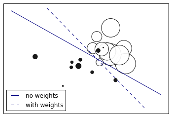
四、考虑权重的二分类

"""
=====================
SGD: Weighted samples
=====================

Plot decision function of a weighted dataset, where the size of points
is proportional to its weight.
"""
print(__doc__)

import numpy as np
import matplotlib.pyplot as plt
from sklearn import linear_model

# we create 20 points
np.random.seed(0)
X = np.r_[np.random.randn(10, 2) + [1, 1], np.random.randn(10, 2)]
y = [1] * 10 + [-1] * 10
sample_weight = 100 * np.abs(np.random.randn(20))
# and assign a bigger weight to the last 10 samples
sample_weight[:10] *= 10

# plot the weighted data points
xx, yy = np.meshgrid(np.linspace(-4, 5, 500), np.linspace(-4, 5, 500))
plt.figure()
plt.scatter(X[:, 0], X[:, 1], c=y, s=sample_weight, alpha=0.9, cmap=plt.cm.bone)　　#散点图

## fit the unweighted model
clf = linear_model.SGDClassifier(alpha=0.01, n_iter=100)
clf.fit(X, y)
Z = clf.decision_function(np.c_[xx.ravel(), yy.ravel()])
Z = Z.reshape(xx.shape)
no_weights = plt.contour(xx, yy, Z, levels=[0], linestyles=['solid'])

## fit the weighted model
clf = linear_model.SGDClassifier(alpha=0.01, n_iter=100)
clf.fit(X, y, sample_weight=sample_weight)
Z = clf.decision_function(np.c_[xx.ravel(), yy.ravel()])
Z = Z.reshape(xx.shape)
samples_weights = plt.contour(xx, yy, Z, levels=[0], linestyles=['dashed'])

plt.legend([no_weights.collections[0], samples_weights.collections[0]],
           ["no weights", "with weights"], loc="lower left")

plt.xticks(())
plt.yticks(())
plt.show()