线性回归

一、回归问题的定义

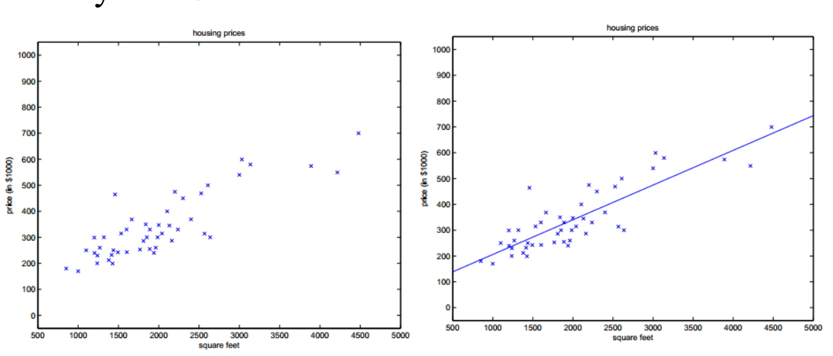
回归是监督学习的一个重要问题，回归用于预测输入变量和输出变量之间的关系。回归模型是表示输入变量到输出变量之间映射的函数。回归问题的学习等价于函数拟合：使用一条函数曲线使其很好的拟合已知函数且很好的预测未知数据。

回归问题分为模型的学习和预测两个过程。基于给定的训练数据集构建一个模型，根据新的输入数据预测相应的输出。

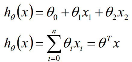
回归问题按照输入变量的个数可以分为一元回归和多元回归；按照输入变量和输出变量之间关系的类型，可以分为线性回归和非线性回归。

 

一元回归：y = ax + b

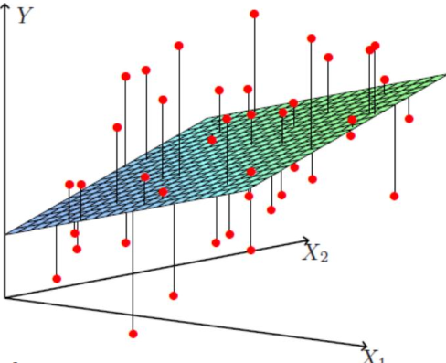
多元回归：

二、回归问题的求解

2.1解析解

2.1.1 最小二乘法

最小二乘法又称最小平方法，它通过最小化误差的平方和寻找数据的最佳函数匹配。利用最小二乘法可以简便地求得未知的数据，并使得这些求得的数据与实际数据之间误差的平方和为最小。最小二乘法还可用于曲线拟合。

2.1.2利用极大似然估计解释最小二乘法

现在假设我们有m个样本，我们假设有：

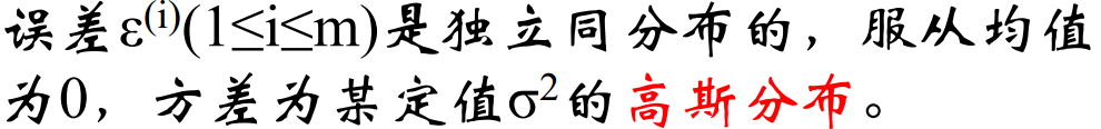
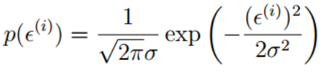
误差项是IID，根据中心极限定理，由于误差项是好多好多相互独立的因素影响的综合影响，我们有理由假设其服从高斯分布，又由于可以自己适配theta0，是的误差项的高斯分布均值为0，所以我们有

所以我们有：

也即：

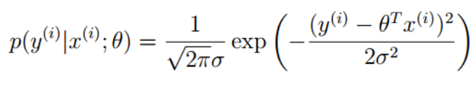 表示在theta给定的时候，给我一个x，就给你一个y

那么我们可以写出似然函数：

由极大似然估计的定义，我们需要L(theta)最大，那么我们怎么才能是的这个值最大呢？两边取对数对这个表达式进行化简如下：

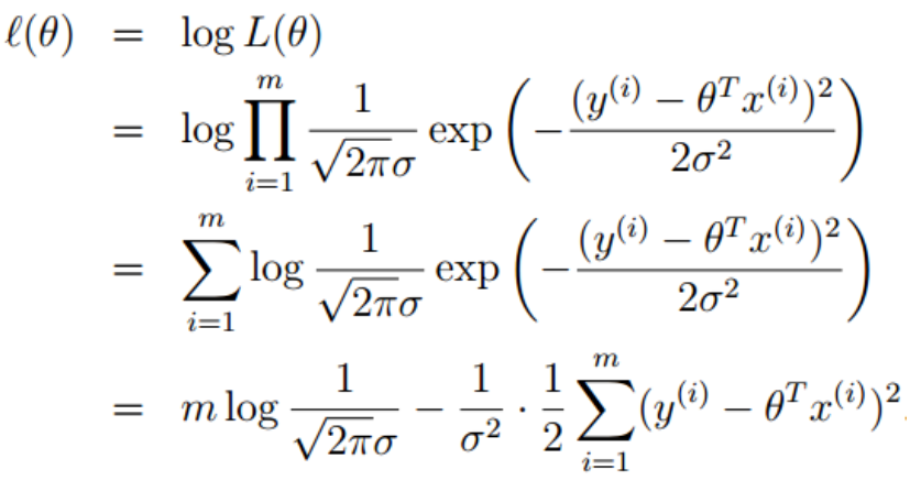
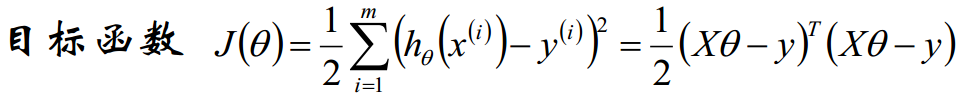
需要 l(theta)最大，也即最后一项的后半部分最小，也即：

所以，我们最后由极大似然估计推导得出，我们希望 J(theta) 最小，而这刚好就是最小二乘法做的工作。而回过头来我们发现，之所以最小二乘法有道理，是因为我们之前假设误差项服从高斯分布，假如我们假设它服从别的分布，那么最后的目标函数的形式也会相应变化。

好了，上边我们得到了有极大似然估计或者最小二乘法，我们的模型求解需要最小化目标函数J(theta)，那么我们的theta到底怎么求解呢？有没有一个解析式可以表示theta?

2.1.3 theta的解析式的求解过程

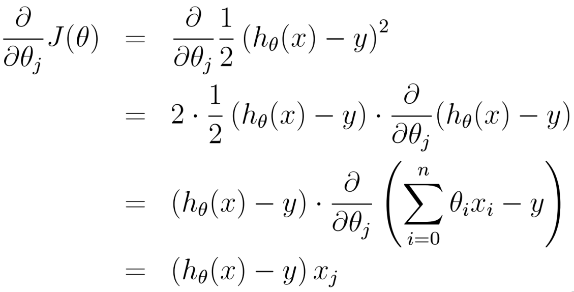
我们需要最小化目标函数，关心 theta 取什么值的时候，目标函数取得最小值，而目标函数连续，那么 theta 一定为 目标函数的驻点，所以我们求导寻找驻点。

求导可得：

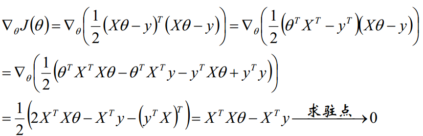
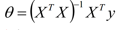
最终我们得到参数 theta 的解析式：

 关于向量、矩阵求导知识参见http://www.cnblogs.com/futurehau/p/6105236.html

上述最后一步有一些问题，假如 X'X不可逆呢？

我们知道 X'X 是一个办正定矩阵，所以若X'X不可逆或为了防止过拟合，我们增加lambda扰动，得到

从另一个角度来看，这相当与给我们的线性回归参数增加一个惩罚因子，这是必要的，我们数据是有干扰的，不正则的话有可能数据对于训练集拟合的特别好，但是对于新数据的预测误差很大。

2.1.4正则化

L2-norm: （Ridge回归）

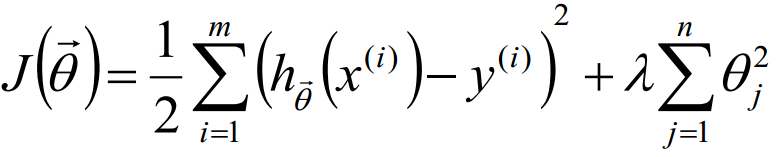
L1-norm: （Lasso回归）

　　J(theta) = J + lambda * sum(|theta|)

L1-norm 和 L2-norm都能防止过拟合，一般L2-norm的效果更好一些。L1-norm能够产生稀疏模型，能够帮助我们去除某些特征，因此可以用于特征选择。

L1-norm 和 L2-norm的直观理解：摘自http://lib.csdn.net/article/machinelearning/42049

 

  

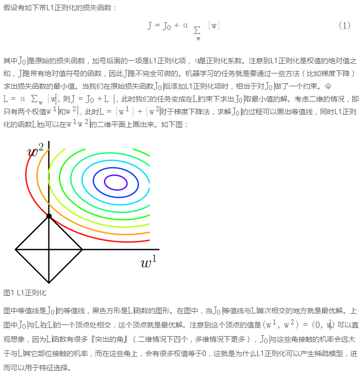
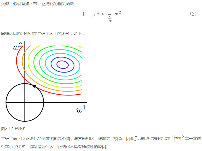
今天又看到一个比较好的解释。可以把加入正则理解为加入约束条件，（类似于逆向拉格朗日）。那么，比如上边的图，L2约束就是一个圆，L1约束就是一个方形。那些关于w的圈圈都是等值线，代表了损失时多少，我们现在要求的就是在约束的条件下寻找最小的损失。所以其实就是找约束的图形和等值线的交点。

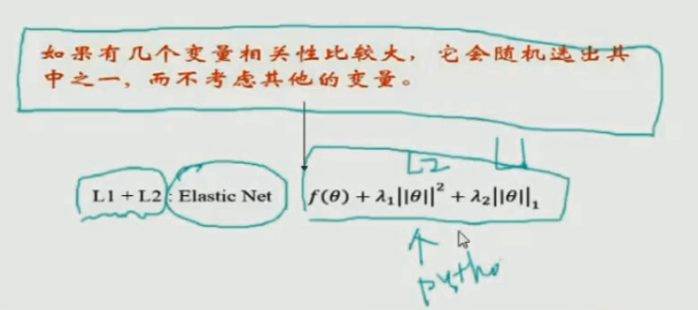
L1的缺点：如果有几个变量相关性比较大，那么它会随机的选择某一个。优化：Elastic Net

 2.2 梯度下降算法

我们在上边给出了最小二乘法求解线性回归的参数theta,实际python 的 numpy库就是使用的这种方法。

当然了，这需要我们的参数的维度不大，当维度大的时候，使用解析解就不适用了，这里讨论梯度下降算法。

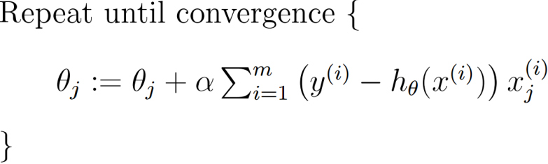
2.2.1梯度下降法步骤：

　　初始化theta

　　沿着负梯度方向迭代，更新后的theta使得J(theta)更小。

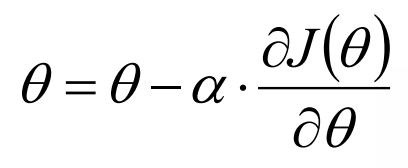
　　其中α表示学习率

　　一个优化技巧：不同的特征采用不同的学习率 Adagrad

　　

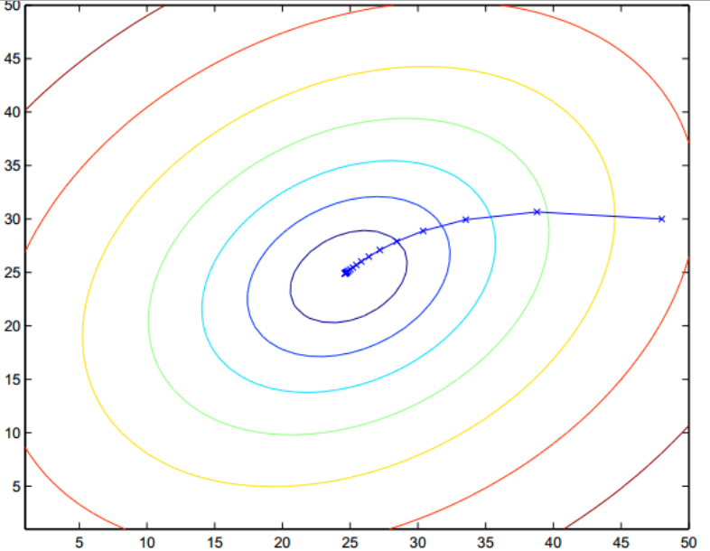
梯度下系那个示意图如下：

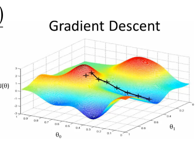
每次迭代找到一个更好的，最后得到一个局部最优解，不一定是全局最优，但是是堪用的。

2.2.2 具体实现

梯度方向：

2.2.2.1 批量梯度下降算法：

由于在线性回归中，目标函数收敛而且为凸函数，是有一个极值点，所以局部最小值就是全局最小值。

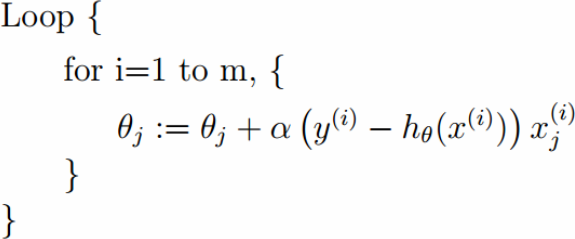
2.2.2.2随机梯度下降算法：

拿到一个样本就下降一次。实际中随机梯度下降算法其实是更适用的。出于一下亮点考虑：

1.由于噪声的存在，不能保证每个变量都让目标函数下降，但总的趋势是下降的。但是另一方面，由于噪声的存在，随机梯度下降算法往往有利于跳出局部最小值。

2.流式数据的处理

2.2.2.3 mini-batch

拿到若干个样本的平均梯度之后在更新梯度方向。

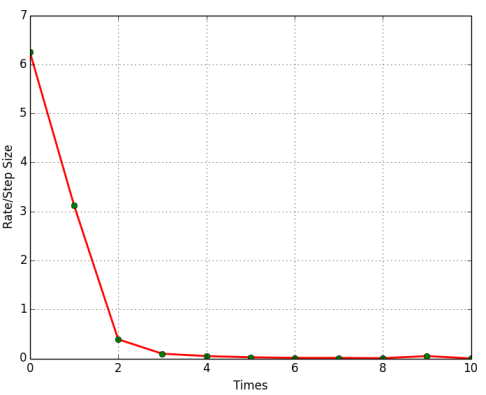
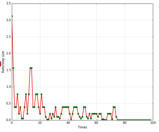
如上图所示，一个批量梯度下降，一个随机梯度下降，最终效果其实是相近的。

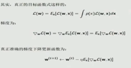
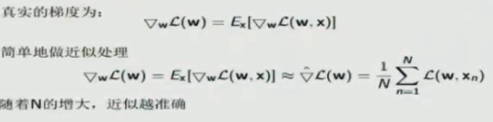
 2.2.2.4 上升一个高度把三种梯度下降算法联系起来

期望损失：理论上模型关于自变量因变量的平均意义下的损失，学习的目标就是选择期望损失最小的模型。

经验风险：模型关于训练样本集的平均损失。因为我们不可能得到所有的样本来计算期望损失，所以我们使用经验风险来代替期望损失。

那么怎么来处理选择这些样本呢？

BGD：我拥有的所有者n个样本的平均损失

SGD:单个样本处理

mini-batch：多个样本处理

 

三、实际线性回归时候的数据使用

此处分析不仅仅局限于线性回归。

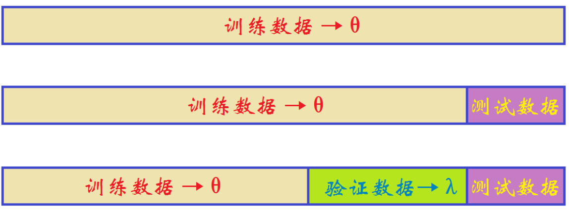
实际中可以把数据分为训练数据和测试数据，然后根据不同模型在测试数据上的表现来选择模型。

另外一些情况，比如上边加上正则化之后，我们不能由训练数据得到lambda，那么我们需要把训练数据进一步划分为训练数据和验证数据。在训练数据上学习theta和lambda，然后在验证数据上选择lambda,然后再在测试数据上验证选择不同模型。

实际中采用交叉验证充分利用数据，例如五折交叉验证。

 

 四、几个系数定义说明

对于m个样本：    

某模型的估计值为： 

定义：

总平方和 TSS(Total Sum of Squares) : 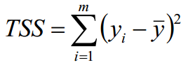 即样本伪方差的m倍 Var(Y) = TSS / m

残差平方和 RSS(Residual Sum of Squares):   RSS也记作误差平方和SSE (Sum of Squares for Error)

可解释平方和ESS(Explained Sum of Squares) :  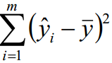ESS又称为回归平方和SSR(Sum of Squares for Regression)

决定系数：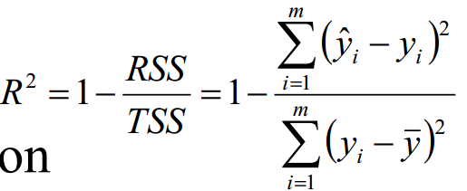

 

TSS >= RSS + ESS， 在无偏估计的时候取等号。

R^2越大，拟合效果越好。

 

需要额外说明的是，这里所谓的线性回归，主要是针对的参数theta,并不是针对x,我们可以对原来的数据进行处理，比如平方得到x^2的数据，然后把这个看作一个影响因素，这样最终得到的y关于x的图形就不是线性的，但当然这也是线性回归。

另外，还有局部加权的线性回归的概念，这部分内容在SVM中进一步解释。

 

五. Linear Regression for binary classfication

考虑到线性分类问题求解不方便，所以可不可以通过线性回归来求解线性分类问题呢？ 

 

 

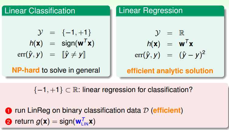
两者的差别主要在于损失函数。

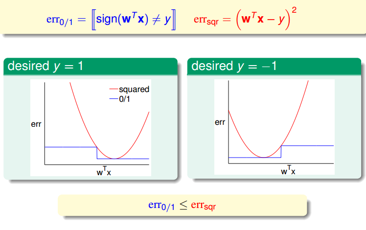
平方损失是0/1损失的一个上限。

所以，使用Linear Regression来求解Linear Regression也是有道理的。

 

使用 sklearn 库来进行训练数据测试数据的划分学习 线性回归库的调用：

#!/usr/bin/python
# -*- coding:utf-8 -*-

import numpy as np
import matplotlib.pyplot as plt
import pandas as pd
from sklearn.model_selection import train_test_split
from sklearn.linear_model import Lasso, Ridge
from sklearn.model_selection import GridSearchCV


if __name__ == "__main__":
    # pandas读入
    data = pd.read_csv('8.Advertising.csv')    # TV、Radio、Newspaper、Sales
    x = data[['TV', 'Radio', 'Newspaper']]
    # x = data[['TV', 'Radio']]
    y = data['Sales']
    print x
    print y

    x_train, x_test, y_train, y_test = train_test_split(x, y, random_state=1)
    # print x_train, y_train
    model = Lasso()
    # model = Ridge()

    alpha_can = np.logspace(-3, 2, 10)  #10^(-3) ~ 10^(2) 等比10个数
    lasso_model = GridSearchCV(model, param_grid={'alpha': alpha_can}, cv=5) #5折交叉验证
    lasso_model.fit(x, y)
    print '验证参数：\n', lasso_model.best_params_

    y_hat = lasso_model.predict(np.array(x_test))
    mse = np.average((y_hat - np.array(y_test)) ** 2)  # Mean Squared Error
    rmse = np.sqrt(mse)  # Root Mean Squared Error
    print mse, rmse

    t = np.arange(len(x_test))
    plt.plot(t, y_test, 'r-', linewidth=2, label='Test')
    plt.plot(t, y_hat, 'g-', linewidth=2, label='Predict')
    plt.legend(loc='upper right')
    plt.grid()
    plt.show()

 

Advertising 完整版代码：

#!/usr/bin/python
# -*- coding:utf-8 -*-

import csv
import numpy as np
import matplotlib.pyplot as plt
import pandas as pd
from sklearn.model_selection import train_test_split
from sklearn.linear_model import LinearRegression


if __name__ == "__main__":
    path = '8.Advertising.csv'
    # # 手写读取数据 - 请自行分析，在8.2.Iris代码中给出类似的例子
    # f = file(path)
    # x = []
    # y = []
    # for i, d in enumerate(f):
    #     if i == 0: #第一行是标题栏
    #         continue
    #     d = d.strip() #去除首位空格
    #     if not d:
    #         continue
    #     d = map(float, d.split(',')) #每个数据都变为float
    #     x.append(d[1:-1])
    #     y.append(d[-1])
    # print x
    # print y
    # x = np.array(x) #显示的更好看
    # y = np.array(y)
    # print x
    # print y

    # # Python自带库
    # f = file(path, 'rb')
    # print f
    # d = csv.reader(f)
    # for line in d:
    #     print line
    # f.close()

    # # numpy读入
    # p = np.loadtxt(path, delimiter=',', skiprows=1)
    # print p
    # print p.shape
    # print p[1,2]
    # print type(p[1,2])

    # pandas读入
    data = pd.read_csv(path)    # TV、Radio、Newspaper、Sales
    # x = data[['TV', 'Radio', 'Newspaper']]
    x = data[['TV', 'Radio']]
    y = data['Sales']
    # print x
    # print y

    # 绘制1
    plt.plot(data['TV'], y, 'ro', label='TV')
    plt.plot(data['Radio'], y, 'g^', label='Radio')
    plt.plot(data['Newspaper'], y, 'mv', label='Newspaer')
    plt.legend(loc='lower right')
    plt.grid()
    plt.show()

    # 绘制2
    plt.figure(figsize=(9,12)) #设置图的大小 宽9inch 高12inch
    plt.subplot(311)
    plt.plot(data['TV'], y, 'ro')
    plt.title('TV')
    plt.grid()
    plt.subplot(312)
    plt.plot(data['Radio'], y, 'g^')
    plt.title('Radio')
    plt.grid()
    plt.subplot(313)
    plt.plot(data['Newspaper'], y, 'b*')
    plt.title('Newspaper')
    plt.grid()
    plt.tight_layout() # 紧凑显示图片，居中显示
    plt.show()

    x_train, x_test, y_train, y_test = train_test_split(x, y, train_size = 0.75, random_state=1) #random_state 种子
    # print x_train, y_train
    linreg = LinearRegression()
    model = linreg.fit(x_train, y_train)
    print model
    print linreg.coef_ #系数
    print linreg.intercept_ #截距

    y_hat = linreg.predict(np.array(x_test))
    mse = np.average((y_hat - np.array(y_test)) ** 2)  # Mean Squared Error
    rmse = np.sqrt(mse)  # Root Mean Squared Error
    print mse, rmse

    t = np.arange(len(x_test))
    plt.plot(t, y_test, 'r-', linewidth=2, label='Test')
    plt.plot(t, y_hat, 'g-', linewidth=2, label='Predict')
    plt.legend(loc='upper right')
    plt.grid()
    plt.show()

 

Advertising 正则化 交叉验证相关代码：

 

线性回归多项式拟合：

#!/usr/bin/python
# -*- coding:utf-8 -*-

import numpy as np
from sklearn.linear_model import LinearRegression, RidgeCV
from sklearn.preprocessing import PolynomialFeatures
import matplotlib.pyplot as plt
from sklearn.pipeline import Pipeline
import matplotlib as mpl


if __name__ == "__main__":
    np.random.seed(0) # 指定种子
    N = 9
    x = np.linspace(0, 6, N) + np.random.randn(N)
    x = np.sort(x)
    y = x**2 - 4*x - 3 + np.random.randn(N)
    # print x
    # print y
    x.shape = -1, 1
    y.shape = -1, 1
    # print x
    # print y

    model_1 = Pipeline([
        ('poly', PolynomialFeatures()),
        ('linear', LinearRegression(fit_intercept=False))])
    model_2 = Pipeline([
        ('poly', PolynomialFeatures()),
        ('linear', RidgeCV(alphas=np.logspace(-3, 2, 100), fit_intercept=False))])
    models = model_1, model_2
    mpl.rcParams['font.sans-serif'] = [u'simHei']
    mpl.rcParams['axes.unicode_minus'] = False
    np.set_printoptions(suppress=True)

    plt.figure(figsize=(9, 11), facecolor='w')
    d_pool = np.arange(1, N, 1)  # 阶
    m = d_pool.size
    clrs = []  # 颜色
    for c in np.linspace(16711680, 255, m):
        clrs.append('#%06x' % c)
    line_width = np.linspace(5, 2, m)
    titles = u'线性回归', u'Ridge回归'
    for t in range(2):
        model = models[t]
        plt.subplot(2, 1, t+1)
        plt.plot(x, y, 'ro', ms=10, zorder=N)
        for i, d in enumerate(d_pool):
            model.set_params(poly__degree=d)
            model.fit(x, y)
            lin = model.get_params('linear')['linear']
            if t == 0:
                print u'%d阶，系数为：' % d, lin.coef_.ravel()
            else:
                print u'%d阶，alpha=%.6f，系数为：' % (d, lin.alpha_), lin.coef_.ravel()
            x_hat = np.linspace(x.min(), x.max(), num=100)
            x_hat.shape = -1, 1
            y_hat = model.predict(x_hat)
            s = model.score(x, y)
            print s, '\n'
            zorder = N - 1 if (d == 2) else 0
            plt.plot(x_hat, y_hat, color=clrs[i], lw=line_width[i], label=(u'%d阶，score=%.3f' % (d, s)), zorder=zorder)
        plt.legend(loc='upper left')
        plt.grid(True)
        plt.title(titles[t], fontsize=16)
        plt.xlabel('X', fontsize=14)
        plt.ylabel('Y', fontsize=14)
    plt.tight_layout(1, rect=(0, 0, 1, 0.95))
    plt.suptitle(u'多项式曲线拟合', fontsize=18)
    plt.show()

 

不使用库：

BGD 与 SGD:

# -*- coding: cp936 -*-
import numpy as np
import matplotlib.pyplot as plt


def linear_regression_BGD(x, y, alpha, lamda):
    m = np.alen(x)
    ones = np.ones(m)
    x = np.column_stack((ones, x))
    n = np.alen(x[0])
    theta = np.ones(n)
    x_traverse = np.transpose(x)

    for i in range(1000):
        hypothesis = np.dot(x, theta)
        loss = hypothesis - y
        cost = np.sum(loss ** 2)
        print i, cost
        gradient = np.dot(x_traverse, loss)
        theta = theta - alpha * gradient
    return theta

def liear_regression_SGD(x, y, alpha, lamda):
    m = np.alen(x)
    ones = np.ones(m)
    x = np.column_stack((ones, x))
    n = np.alen(x[0])
    theta = np.ones(n)
    for j in range(1, m):
        hypothesis = np.dot(x[j], theta)
        loss = hypothesis - y[j]
        gradient = np.dot(loss, x[j])
        theta = theta - alpha * gradient
    return theta



if __name__ == '__main__':
    N = 10
    # x = np.linspace(0, 10, N) + np.random.randn(N)
    # y =  3 * x + 5 + np.random.randn(N)

    x = np.linspace(0, 10, N) + np.random.randn(N)
    y = 4 * x * x + 3 * x + 5 + np.random.randn(N)
    x_square = x * x
    x_predict = np.column_stack((x, x_square))

    # theta = linear_regression_BGD(x_predict, y, 0.00001,0.1) # 批量梯度下降
    theta = liear_regression_SGD(x_predict, y, 0.0001, 0.1) # 随机梯度下降
    plt.plot(x, y, 'ro')

    x = np.linspace(x.min(), x.max(), 10 * N) # 构建测试数据
    ones = np.ones(10 * N)
    # x_predict = np.column_stack((ones, x))x
    x_test = np.column_stack((ones, x, x * x))
    y = np.dot(x_test, theta)

    plt.plot(x, y, 'b-')
    plt.show()

 

Regression代码：

import numpy as np
import matplotlib.pyplot as plt
def regression(data, alpha, lamda ):
    n = len(data[0]) - 1
    theta = np.zeros(n)
    times = 1
    for i in range(times):
        for d in data:
            x = d[:-1]
            y = d[-1]
            h_theta = np.dot(theta, x) - y
            theta = theta - alpha * h_theta * x + lamda * theta
        #print i,theta
    return theta
def preduceData():
   x = []
   y = []
   for i in range(0, 50):
       x.append(i)
       y.append(3 * x[i] + np.random.random_sample()*3)
   data = np.array([x, y]).T
   theta = regression(data, 0.001, 0.1)
   return x, y, theta
def myplot(x, y, theta):
    plt.figure()
    plt.plot(x, y, 'go')
    plt.plot(x, theta * x, 'r')
    plt.show()
x, y, theta = preduceData()
myplot(x, y, theta)