Exercise: Logistic Regression and Newton's Method

题目地址：

题目概要：某个高中有80名学生，其中40名得到了大学的录取，40名没有被录取。x中包含80名学生两门标准考试的成绩，y中包含学生是否被录取（1代表录取、0代表未录取）。

过程：

1、加载试验数据，并为x输入添加一个偏置项。

x=load('ex4x.dat');
y=load('ex4y.dat');
x=[ones(length(y),1) x];

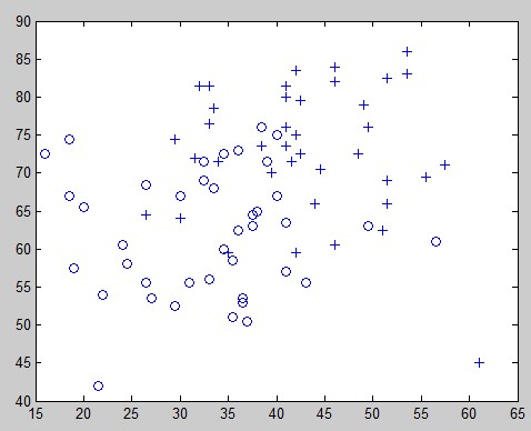
2、绘制数据分布

 % find returns the indices of the
% rows meeting the specified condition
pos = find(y == 1); neg = find(y == 0);

% Assume the features are in the 2nd and 3rd
% columns of x
plot(x(pos, 2), x(pos,3), '+'); hold on
plot(x(neg, 2), x(neg, 3), 'o')

3、Newton's method

先回忆一下logistic regression的假设：

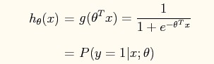
因为matlab中没有sigmoid函数，因此我们用niline定义一个：

g = inline('1.0 ./ (1.0 + exp(-z))'); 
% Usage: To find the value of the sigmoid 
% evaluated at 2, call g(2)

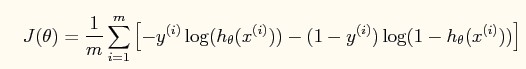
再来看看我们定义的cost function J(θ):

我们希望使用Newton's method来求出cost function J(θ)的最小值。回忆一下Newton's method中θ的迭代规则为：

在logistic regression中，梯度和Hessian的求法分别为：

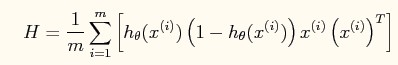
需要注意的是，上述公式中的写法为向量形式。

其中，为n+1 * 1的向量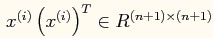，为n+1 * n+1的矩阵。

和为标量。

实现

按照上述Newton's method所述的方法逐步实现。代码如下

function [theta, J ] = newton( x,y )
%NEWTON Summary of this function goes here
%   Detailed explanation goes here
m = length(y);
theta = zeros(3,1);
g = inline('1.0 ./ (1.0 + exp(-z))'); 
pos = find(y == 1);
neg = find(y == 0);
J = zeros(10, 1); 
for num_iterations = 1:10
    %计算实际输出
    h_theta_x = g(x * theta);
    %将y=0和y=1的情况分开计算后再相加，计算J函数
    pos_J_theta = -1 * log(h_theta_x(pos));
    neg_J_theta = -1 *log((1- h_theta_x(neg)));
    J(num_iterations) = sum([pos_J_theta;neg_J_theta])/m;
    %计算J导数及Hessian矩阵
    delta_J = sum(repmat((h_theta_x - y),1,3).*x);
    H = x'*(repmat((h_theta_x.*(1-h_theta_x)),1,3).*x);
    %更新θ
    theta = theta - inv(H)*delta_J';
end
% now plot J
% technically, the first J starts at the zero-eth iteration
% but Matlab/Octave doesn't have a zero index
figure;
plot(0:9, J(1:10), '-')
xlabel('Number of iterations')
ylabel('Cost J')
end

PS：在练习的附录答案中给出的直接计算J函数的代码很优雅：

J(i) =(1/m)*sum(-y.*log(h) - (1-y).*log(1-h));

在matlab中调用：

[theta J] = newton(x,y);

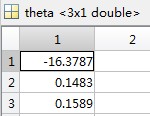
可以得到输出：

θ为：

J函数输出图像为（令迭代次数为10的情况下）：

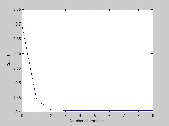
可以看到，其实在迭代至第四次时，就已经收敛了。

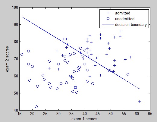
我们可以输出一下admitted和unadmitted的分界线，代码如下：

 plot(x(pos, 2), x(pos,3), '+'); hold on
plot(x(neg, 2), x(neg, 3), 'o')
ylabel('exam 2 scores')
xlabel('exam 1 scores')
plot(x(:,2), (theta(1) - x(:,2)*theta(2))/theta(3), '-');
legend('admitted', 'unadmitted','decision boundary');