
在 Spark 中使用 IPython Notebook
本文是从 IPython Notebook 转化而来,效果没有本来那么好。
主要为体验 IPython Notebook。至于题目,改成《在 IPython Notebook 中使用 Spark》也可以,没什么差别。为什么是 Spark?因为这两天在看《Spark 机器学习》这本书第 3 章,所以就顺便做个笔记。
简单介绍下,IPython notebook 对数据科学家来说是个交互地呈现科学和理论工作的必备工具,它集成了文本和 Python 代码。Spark 是个通用的集群计算框架,通过将大量数据集计算任务分配到多台计算机上,提供高效内存计算。
搭建环境
一台阿里云服务器,配置如下,108 元/月,然后在 Windows 7 上使用 Putty 和远程桌面操作服务器。
CPU:1核
内存:2048 MB
操作系统:Ubuntu 14.04 64位
固定带宽:1Mbps
IPython Notebook 的安装很简单,强烈推荐一个预编译的科学 Python 套件 Anaconda,按照官方网站安装,然后在 Terminal 里执行 ipython notebook 即可。
在我的 Ubuntu 服务器上打开 ipython notebook 时报错了:socket.error Errno 99 Cannot assign requested address。
这个问题耗了我一天时间。关于这个问题,众 说 纷 纭,但只有下面两种方法管用。
一种是,在命令后加参数 --ip:ipython notebook --ip=127.0.0.1。
另一种是,先生成 notebook 配置文件:命令行执行 jupyter notebook --generate-config,然后打开生成的文件: vi ~/.jupyter/jupyter_notebook_config.py,修改 c.NotebookApp.ip = '127.0.0.1'。
如果想外网也可以访问,ip 就设为外网 IP 地址。我选择的是第二种,设的外网 IP 地址,这样就可以在 Windows 上编辑 ipython notebook 文件了,非常方便。

Spark 的安装也很简单,具体安装和使用可参考我之前的笔记和官方网站。
如何在 Spark 中使用 IPython Notebook,或者如何在 IPython Notebook 中使用 spark,也耗费了我一天时间。
网上很多文章都是建议:1、执行 ipython profile create spark;2、创建 ~/.ipython/profile_spark/startup/00-pyspark-setup.py 文件并修改;3、启动 IPython notebook:ipython notebook --profile spark。
但这种方法在我这行不通,百般折腾,就是各种不行。
后来终于发现一种简单可行的方法,那就是修改 ~/.bashrc 文件,添加以下内容:
export PYSPARK_DRIVER_PYTHON=ipython2 # As pyspark only works with python2 and not python3
export PYSPARK_DRIVER_PYTHON_OPTS="notebook"
然后source .bashrc,就可以通过启动 pyspark 来启动 IPython Notebook 了。也就可以在 IPython Notebook 中使用 pyspark 了。
下面我们通过实例演示 Spark 在 IPython Notebook 中的使用。
Spark 上数据的探索和处理
MovieLens 100k 数据集
这里要使用的是著名的 MovieLens 100k 数据集,该数据集包含用户对电影的 10 万次评分数据,也包含电影元数据和用户属性数据。数据集不大,压缩文件不到 5M,常用于推荐系统研究。
可到官方网站下载,解压后会创建一个名为 ml-100k 的文件夹,该目录中重要的文件有 u.user(用户属性文件)、u.item(电影元数据) 和 u.data(用户对电影的评分)。
数据集的更多信息可以从 README 获得,包括每个数据文件里的变量定义。我们可以使用 head 命令来查看各个文件的内容。
先来看 u.user:
#head -5 u.user
1|24|M|technician|85711
2|53|F|other|94043
3|23|M|writer|32067
4|24|M|technician|43537
5|33|F|other|15213
可以看到 u.user 文件包含 user id、age、gender、occupation 和 ZIP code 这些属性,各属性之间用管道符(|)隔开。
再来看 u.item:
# head -5 u.item
1|Toy Story (1995)|01-Jan-1995||http://us.imdb.com/M/title-exact?Toy%20Story%20(1995)|0|0|0|1|1|1|0|0|0|0|0|0|0|0|0|0|0|0|0
2|GoldenEye (1995)|01-Jan-1995||http://us.imdb.com/M/title-exact?GoldenEye%20(1995)|0|1|1|0|0|0|0|0|0|0|0|0|0|0|0|0|1|0|0
3|Four Rooms (1995)|01-Jan-1995||http://us.imdb.com/M/title-exact?Four%20Rooms%20(1995)|0|0|0|0|0|0|0|0|0|0|0|0|0|0|0|0|1|0|0
4|Get Shorty (1995)|01-Jan-1995||http://us.imdb.com/M/title-exact?Get%20Shorty%20(1995)|0|1|0|0|0|1|0|0|1|0|0|0|0|0|0|0|0|0|0
5|Copycat (1995)|01-Jan-1995||http://us.imdb.com/M/title-exact?Copycat%20(1995)|0|0|0|0|0|0|1|0|1|0|0|0|0|0|0|0|1|0|0
u.item 文件包含 movie id、title、release date 以及若干与 IMDB Link 和电影分类相关的属性,各属性之间也用 | 符号分隔。电影分类的属性有 unknown | Action | Adventure | Animation | Children's | Comedy | Crime | Documentary | Drama | Fantasy | Film-Noir | Horror | Musical | Mystery | Romance | Sci-Fi | Thriller | War | Western。
最后 u.data:
# head -5 u.data
196 242 3 881250949
186 302 3 891717742
22 377 1 878887116
244 51 2 880606923
166 346 1 886397596
u.data 文件包含 user id、movie id、rating(从 1 到 5)和 timestamp 属性。各属性间用指标符分隔。timestamp 是从 1/1/1970 UTC 开始的秒数。
探索与可视化数据集
先来探索用户数据。
user_data = sc.textFile("ml-100k/u.user")
user_data.first()  #此处如能输出数据文件首行,则说明环境搭建没问题
u'1|24|M|technician|85711'
sc 是 Spark shell 启动时自动创建的一个 SparkContext 对象,shell 通过该对象来访问 Spark。可以通过下列方法输出 sc 来查看它的类型。
sc
<pyspark.context.SparkContext at 0x7fb65c173450>
一旦有了 SparkContext,你就可以用它来创建 RDD。RDD 是弹性分布式数据集(Resilient Distributed Dataset),在 Spark 中,我们通过对 RDD 的操作来表达我们的计算意图,这些计算会自动地在集群上并行进行。
如上面代码创建了一个名为 user_data 的 RDD,然后使用 user_data.first() 输出了 RDD 中的第一个元素。
下面用“|”字符来分隔各行数据。这将生成一个 RDD,其中每一个记录对应一个 Python 列表,各列表由用户 ID、年龄、性别、职业和邮编五个属性构成。之后再统计用户、性别、职业和邮编的数目。可通过下列代码实现。
user_fields = user_data.map(lambda line: line.split("|"))
num_users = user_fields.map(lambda fields: fields[0]).count()
num_genders = user_fields.map(lambda fields: fields[2]).distinct().count()
num_occupations = user_fields.map(lambda fields: fields[3]).distinct().count()
num_zipcodes = user_fields.map(lambda fields: fields[4]).distinct().count()
print "Users: %d, genders: %d, occupations: %d, ZIP codes: %d" % (num_users, num_genders, num_occupations, num_zipcodes)
Users: 943, genders: 2, occupations: 21, ZIP codes: 795
接着用 Matplotlib 的 hist 函数来创建一个直方图,以分析用户年龄的分布情况。
%pylab inline
Populating the interactive namespace from numpy and matplotlib
ages = user_fields.map(lambda x: int(x[1])).collect()
hist(ages, bins=20, color='lightblue', normed=True)
fig = matplotlib.pyplot.gcf()
fig.set_size_inches(16, 10)

这里 hist 函数的输入参数有 ages 数组、直方图的 bins 数目(即区间数,这里为 20),同时,还使用了 normed=True 参数来正则化直方图,即让每个方条表示年龄在该区间内的数量占总数量的比。
从中可以看出 MovieLens 的大量用户处于 15 到 55 之间。
若想了解用户的职业分布情况,可以用如下代码来实现。首先利用 MapReduce 方法来计算数据集中各种职业的出现次数,然后用 matplotlib 的 bar 函数来会绘制一个不同职业的数量的条形图。
count_by_occupation = user_fields.map(lambda fields: (fields[3], 1)).reduceByKey(lambda x, y: x + y).collect()
x_axis1 = np.array([c[0] for c in count_by_occupation])
y_axis1 = np.array([c[1] for c in count_by_occupation])
x_axis = x_axis1[np.argsort(y_axis1)]
y_axis = y_axis1[np.argsort(y_axis1)]

pos = np.arange(len(x_axis))
width = 1.0

ax = plt.axes()
ax.set_xticks(pos + (width / 2))
ax.set_xticklabels(x_axis)

plt.bar(pos, y_axis, width, color='lightblue')
plt.xticks(rotation=30)
fig = matplotlib.pyplot.gcf()
fig.set_size_inches(16, 10)

count_by_occupation
[(u'administrator', 79),
 (u'writer', 45),
 (u'retired', 14),
 (u'student', 196),
 (u'doctor', 7),
 (u'entertainment', 18),
 (u'marketing', 26),
 (u'executive', 32),
 (u'none', 9),
 (u'scientist', 31),
 (u'educator', 95),
 (u'lawyer', 12),
 (u'healthcare', 16),
 (u'technician', 27),
 (u'librarian', 51),
 (u'programmer', 66),
 (u'artist', 28),
 (u'salesman', 12),
 (u'other', 105),
 (u'homemaker', 7),
 (u'engineer', 67)]
x_axis1
array([u'administrator', u'writer', u'retired', u'student', u'doctor',
       u'entertainment', u'marketing', u'executive', u'none', u'scientist',
       u'educator', u'lawyer', u'healthcare', u'technician', u'librarian',
       u'programmer', u'artist', u'salesman', u'other', u'homemaker',
       u'engineer'],
      dtype='<U13')
y_axis1
array([ 79,  45,  14, 196,   7,  18,  26,  32,   9,  31,  95,  12,  16,
        27,  51,  66,  28,  12, 105,   7,  67])
从中可以看出,数量最多的职业是 student、other、educator、administrator、engineer 和 programmer。
Spark 对 RDD 提供了一个名为 countByValue 的便捷函数,它会计算 RDD 里各不同值所分别出现的次数,并将其以 Python dict 函数的形式返回给驱动程序。
count_by_occupation2 = user_fields.map(lambda fields: fields[3]).countByValue()
print "Map-reduce approach:"
print dict(count_by_occupation2)
print ""
print "countByValue approach:"
print dict(count_by_occupation)
Map-reduce approach:
{u'administrator': 79, u'retired': 14, u'lawyer': 12, u'healthcare': 16, u'marketing': 26, u'executive': 32, u'scientist': 31, u'student': 196, u'technician': 27, u'librarian': 51, u'programmer': 66, u'salesman': 12, u'homemaker': 7, u'engineer': 67, u'none': 9, u'doctor': 7, u'writer': 45, u'entertainment': 18, u'other': 105, u'educator': 95, u'artist': 28}

countByValue approach:
{u'administrator': 79, u'executive': 32, u'retired': 14, u'doctor': 7, u'entertainment': 18, u'marketing': 26, u'writer': 45, u'none': 9, u'healthcare': 16, u'scientist': 31, u'homemaker': 7, u'student': 196, u'educator': 95, u'technician': 27, u'librarian': 51, u'programmer': 66, u'artist': 28, u'salesman': 12, u'other': 105, u'lawyer': 12, u'engineer': 67}
可以看到,上述两种方式的结果相同。
接下来探索电影数据,跟之前一样,先简单看下第一行记录,然后再统计电影总数。
movie_data = sc.textFile("ml-100k/u.item")
print movie_data.first()
num_movies = movie_data.count()
print "Movies: %d" % num_movies
1|Toy Story (1995)|01-Jan-1995||http://us.imdb.com/M/title-exact?Toy%20Story%20(1995)|0|0|0|1|1|1|0|0|0|0|0|0|0|0|0|0|0|0|0
Movies: 1682
在此要绘制电影年龄分布图,电影年龄即其发行年份相对于现在过了多少年(在本数据中现在是 1998 年)。电影数据有些不完整,需要一个函数来处理解析 release date 时可能出现的解析错误。这里命名该函数为 convert_year。
def convert_year(x):
    try:
        return int(x[-4:])
    except:
        return 1900 # there is a 'bad' data point with a blank year, which we set to 1900 and will filter out later
有了以上函数来解析发行年份后,便可在调用电影数据进行 map 转换时应用该函数,并取回其结果。
movie_fields = movie_data.map(lambda lines: lines.split("|"))
years = movie_fields.map(lambda fields: fields[2]).map(lambda x: convert_year(x))
# we filter out any 'bad' data points here
years_filtered = years.filter(lambda x: x != 1900)
# plot the movie ages histogram
movie_ages = years_filtered.map(lambda yr: 1998-yr).countByValue()
values = movie_ages.values()
bins = movie_ages.keys()
hist(values, bins=bins, color='lightblue', normed=True)
fig = matplotlib.pyplot.gcf()
fig.set_size_inches(16,10)

从图中可以看到,大部分电影发行于 1998 年的前几年。
现实的数据经常会有不规整的情况,对其解析时就需要进一步处理。上面即是一个很好的例子。事实上,这也表明了数据探索的重要性所在,即它有助于发现数据在完整性和质量上的问题。
现在来探索评级数据:
rating_data_raw = sc.textFile("ml-100k/u.data")
print rating_data_raw.first()
num_ratings = rating_data_raw.count()
print "Ratings: %d" % num_ratings
196	242	3	881250949
Ratings: 100000
可以看到评级次数共有 10 万条。另外和用户与电影数据不同,评分记录用“\t”分隔。
rating_data = rating_data_raw.map(lambda line: line.split("\t"))
ratings = rating_data.map(lambda fields: int(fields[2]))
max_rating = ratings.reduce(lambda x, y: max(x, y))
min_rating = ratings.reduce(lambda x, y: min(x, y))
mean_rating = ratings.reduce(lambda x, y: x + y) / float(num_ratings)
median_rating = np.median(ratings.collect())
ratings_per_user = num_ratings / num_users
ratings_per_movie = num_ratings / num_movies
print "Min rating: %d" % min_rating
print "Max rating: %d" % max_rating
print "Average rating: %2.2f" % mean_rating
print "Median rating: %d" % median_rating
print "Average # of ratings per user: %2.2f" % ratings_per_user
print "Average # of ratings per movie: %2.2f" % ratings_per_movie
Min rating: 1
Max rating: 5
Average rating: 3.53
Median rating: 4
Average # of ratings per user: 106.00
Average # of ratings per movie: 59.00
从中可以看到,最低的评级为 1,而最大的评级为 5.这并不意外,因为评级的范围便是从 1 到 5。
Spark 对 RDD 也提供一个名为 states 的函数。该函数包含一个数值变量用于做类似的统计:
ratings.stats()
(count: 100000, mean: 3.52986, stdev: 1.12566797076, max: 5.0, min: 1.0)
可以看出,用户对电影的平均评级是 3.5 左右,而评分中位数为 4,。说明评级的分布稍倾向高分。要验证这点,可创建一个评级值分布的条形图。
# create plot of counts by rating value
count_by_rating = ratings.countByValue()
x_axis = np.array(count_by_rating.keys())
y_axis = np.array([float(c) for c in count_by_rating.values()])
# we normalize the y-axis here to percentages
y_axis_normed = y_axis / y_axis.sum()

pos = np.arange(len(x_axis))
width = 1.0

ax = plt.axes()
ax.set_xticks(pos + (width / 2))
ax.set_xticklabels(x_axis)

plt.bar(pos, y_axis_normed, width, color='lightblue')
plt.xticks(rotation=30)
fig = matplotlib.pyplot.gcf()
fig.set_size_inches(16, 10)

其特征和之前的期待相同,评分分布确实偏向中等以上。
同样,也可以求各个用户评级次数的分布情况。计算各用户评级次数的分布时,先从 rating_data RDD 里提取出以用户 ID 为主键、评级为值的键值对。之后调用 Spark 的 groupByKey 函数,来对评级以用户 ID 为主键进行分组。
# to compute the distribution of ratings per user, we first group the ratings by user id
user_ratings_grouped = rating_data.map(lambda fields: (int(fields[0]), int(fields[2]))).groupByKey()
接着求出每一个主键(用户 ID)对应的评级集合的大小,这会给出各用户评级的次数:
# then, for each key (user id), we find the size of the set of ratings, which gives us the # ratings for that user
user_ratings_byuser = user_ratings_grouped.map(lambda (k, v): (k, len(v)))
user_ratings_byuser.take(5)
[(1, 272), (2, 62), (3, 54), (4, 24), (5, 175)]
最后,用 hist 来绘制用户评级分布的直方图。
# and finally plot the histogram
user_ratings_byuser_local = user_ratings_byuser.map(lambda (k, v): v).collect()
hist(user_ratings_byuser_local, bins=200, color='lightblue', normed=True)
fig = matplotlib.pyplot.gcf()
fig.set_size_inches(16,10)
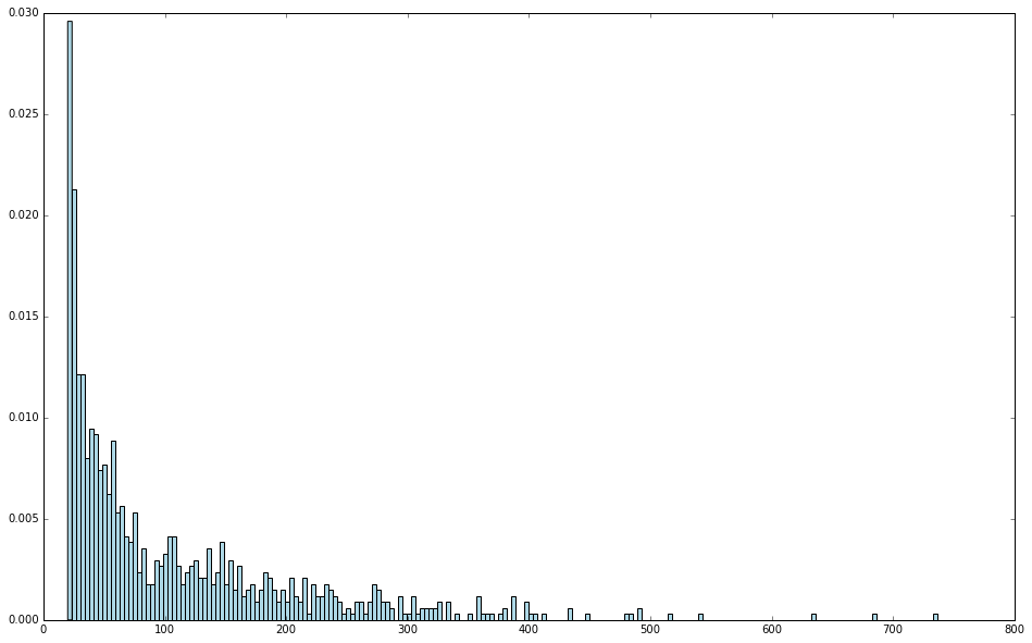
可以看出,大部分用户的评级次数少于 100,但也表明仍然有较多用户做出过上百次的评级。

 浙公网安备 33010602011771号