支持向量机（SVM）

简介

SVM是支持向量机（Support Vector Machines）的简称，是一种二分类模型。

支持向量机所做的就是去寻找两类数据的分隔线，通常将这个分隔线叫做超平面。

分隔的原则是间隔最大化，最终转化为一个凸二次规划问题来求解。

基本思想

（1）线性分割

如果一个线性函数能够将样本（比如说两类点）分开，那么称这些数据样本是线性可分的

线性函数在二维空间就是一条直线，在三维空间就是一个平面，在不考虑维数的情况下线性函数统称为超平面。

如图：实心点和空心点是两类点

这两类点，有无数条直线可以将它们分隔开

SVM的目标就是在这无数条线中，找出一条线使这条线与两类样本（两类点）中最近的点距离最大

这个距离叫做间隔

但有时因为数据的问题不能画出分割线时，例如这样：

很显然，分隔线是不存在的，这时可以将这个点当作异常来处理

即忽略这个点，再分割

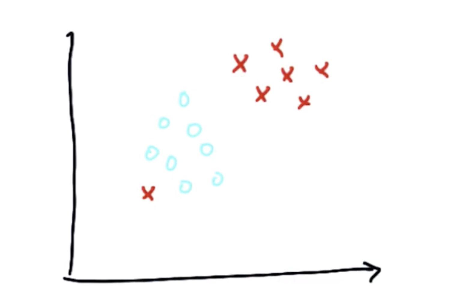
（2）非线性分割

还有一些数据是用一条直线分割不出来的，就像这样：

在线性分割时，我们向SVM提供样本的坐标数据（X，Y）即X和Y来进行计算

针对图中的情况，我们可以引入第三个数据Z，令Z = X^2 + Y^2

再画出Z-X图：

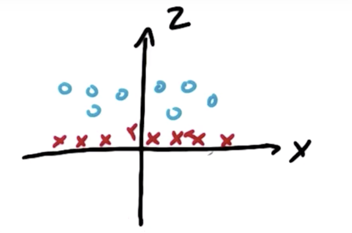
通过这一转化，就可以针对Z，X进行分割

再一个例子

样本无法直接根据X，Y来划分，此时将样本的坐标转化为 |X|，Y 画出图像：

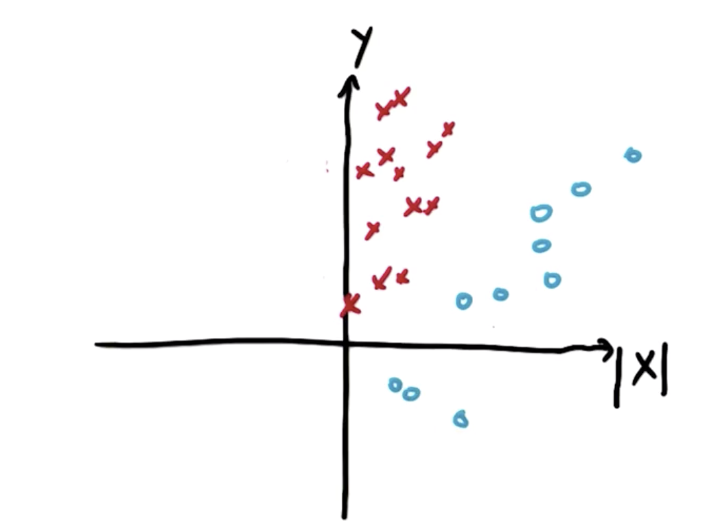
即可划分

（3）核技巧（Kernel Trick）

核函数即是接受低纬度的输入空间或者特征空间，并将其映射到高维度空间，所以过去不可以线性分割的内容变为可分割的。

应用核函数技巧将输入空间从x,y变到更大的输入空间后，再使用支持向量机对数据点进行分类，得到解后返回原始空间

这样就得到了一个非线性分割

核函数有很多种，其中常用的有：

linear（线性），ploy（多项式），rbf（径向基函数），sigmoid（s函数）

在SVM算法中，核函数作为一个参数发挥作用

（4）其他参数（C、gamma）

不仅是核作为参数影响SVM分割，还有其他参数，例如C和Gamma，其中C的影响最大，Gamma几乎没有影响

C的作用：在光滑的决策边界以及尽可能正确分类所有训练点之间进行平衡（C越大正确点越多），但代价时模型更复杂

　　　　　C=10000,kernal='rbf'　　　　　　　　　　　　　　　C=10 kernel='rbf'

C=10000,kernal='rbf'

如图核函数相同时，C相差三个数量级时的区别

通过调整核函数，C和Gamma来避免过拟合现象

代码实现

环境：MacOS mojave　　10.14.3

Python　　3.7.0

使用库：scikit-learn 0.19.2

sklearn.SVM库官方文档：https://scikit-learn.org/dev/modules/generated/sklearn.svm.SVC.html

>>> import numpy as np
>>> X = np.array([[-1, -1], [-2, -1], [1, 1], [2, 1]])#生成四个训练点
>>> y = np.array([1, 1, 2, 2])#前两个点分为标签1，后两个点分为标签2
>>> from sklearn.svm import SVC
>>> clf = SVC(gamma='auto')#默认核函数线性分割
>>> clf.fit(X, y) #训练
SVC(C=1.0, cache_size=200, class_weight=None, coef0=0.0,
    decision_function_shape='ovr', degree=3, gamma='auto', kernel='rbf',
    max_iter=-1, probability=False, random_state=None, shrinking=True,
    tol=0.001, verbose=False)#使用rbf核函数，c为1，gamma自动配置
>>> print(clf.predict([[-0.8, -1]]))    #预测新的点
[1]    #结果为标签1

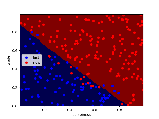
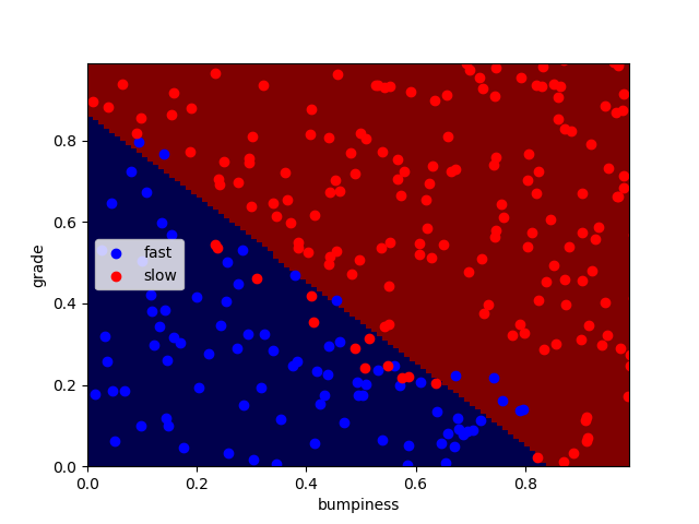
以线性数据举例

Main.py　　主程序

import sys
from class_vis import prettyPicture
from prep_terrain_data import makeTerrainData

import matplotlib.pyplot as plt
import copy
import numpy as np
import pylab as pl


features_train, labels_train, features_test, labels_test = makeTerrainData()


########################## SVM #################################
### we handle the import statement and SVC creation for you here
from sklearn.svm import SVC
clf = SVC(kernel="linear",C = 1000)


#### now your job is to fit the classifier
#### using the training features/labels, and to
#### make a set of predictions on the test data
clf.fit(features_train, labels_train)


#### store your predictions in a list named pred

pred = []
pred = clf.predict(features_test)

prettyPicture(clf, features_test, labels_test)

from sklearn.metrics import accuracy_score
acc = accuracy_score(pred, labels_test)
print(acc)

def submitAccuracy():
    return acc

perp_terrain_data.py　　生成训练点

#!/usr/bin/python
import random


def makeTerrainData(n_points=1000):
###############################################################################
### make the toy dataset
    random.seed(42)
    grade = [random.random() for ii in range(0,n_points)]
    bumpy = [random.random() for ii in range(0,n_points)]
    error = [random.random() for ii in range(0,n_points)]
    y = [round(grade[ii]*bumpy[ii]+0.3+0.1*error[ii]) for ii in range(0,n_points)]
    for ii in range(0, len(y)):
        if grade[ii]>0.8 or bumpy[ii]>0.8:
            y[ii] = 1.0

### split into train/test sets
    X = [[gg, ss] for gg, ss in zip(grade, bumpy)]
    split = int(0.75*n_points)
    X_train = X[0:split]
    X_test  = X[split:]
    y_train = y[0:split]
    y_test  = y[split:]

    grade_sig = [X_train[ii][0] for ii in range(0, len(X_train)) if y_train[ii]==0]
    bumpy_sig = [X_train[ii][1] for ii in range(0, len(X_train)) if y_train[ii]==0]
    grade_bkg = [X_train[ii][0] for ii in range(0, len(X_train)) if y_train[ii]==1]
    bumpy_bkg = [X_train[ii][1] for ii in range(0, len(X_train)) if y_train[ii]==1]

#    training_data = {"fast":{"grade":grade_sig, "bumpiness":bumpy_sig}
#            , "slow":{"grade":grade_bkg, "bumpiness":bumpy_bkg}}


    grade_sig = [X_test[ii][0] for ii in range(0, len(X_test)) if y_test[ii]==0]
    bumpy_sig = [X_test[ii][1] for ii in range(0, len(X_test)) if y_test[ii]==0]
    grade_bkg = [X_test[ii][0] for ii in range(0, len(X_test)) if y_test[ii]==1]
    bumpy_bkg = [X_test[ii][1] for ii in range(0, len(X_test)) if y_test[ii]==1]

    test_data = {"fast":{"grade":grade_sig, "bumpiness":bumpy_sig}
            , "slow":{"grade":grade_bkg, "bumpiness":bumpy_bkg}}

    return X_train, y_train, X_test, y_test
#    return training_data, test_data

class_vis.py　　绘图与保存图像

import warnings
warnings.filterwarnings("ignore")

import matplotlib 
matplotlib.use('agg')

import matplotlib.pyplot as plt
import pylab as pl
import numpy as np

#import numpy as np
#import matplotlib.pyplot as plt
#plt.ioff()

def prettyPicture(clf, X_test, y_test):
    x_min = 0.0; x_max = 1.0
    y_min = 0.0; y_max = 1.0

    # Plot the decision boundary. For that, we will assign a color to each
    # point in the mesh [x_min, m_max]x[y_min, y_max].
    h = .01  # step size in the mesh
    xx, yy = np.meshgrid(np.arange(x_min, x_max, h), np.arange(y_min, y_max, h))
    Z = clf.predict(np.c_[xx.ravel(), yy.ravel()])

    # Put the result into a color plot
    Z = Z.reshape(xx.shape)
    plt.xlim(xx.min(), xx.max())
    plt.ylim(yy.min(), yy.max())

    plt.pcolormesh(xx, yy, Z, cmap=pl.cm.seismic)

    # Plot also the test points
    grade_sig = [X_test[ii][0] for ii in range(0, len(X_test)) if y_test[ii]==0]
    bumpy_sig = [X_test[ii][1] for ii in range(0, len(X_test)) if y_test[ii]==0]
    grade_bkg = [X_test[ii][0] for ii in range(0, len(X_test)) if y_test[ii]==1]
    bumpy_bkg = [X_test[ii][1] for ii in range(0, len(X_test)) if y_test[ii]==1]

    plt.scatter(grade_sig, bumpy_sig, color = "b", label="fast")
    plt.scatter(grade_bkg, bumpy_bkg, color = "r", label="slow")
    plt.legend()
    plt.xlabel("bumpiness")
    plt.ylabel("grade")

    plt.savefig("test.png")

得到结果：正确率92%

以非线性核函数举例

在数据点不变的情况下，使用rbf核，并使C的值设定为1000，10000，100000

clf = SVC(kernel="rbf",C = 100000)

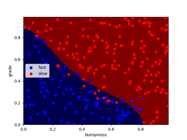
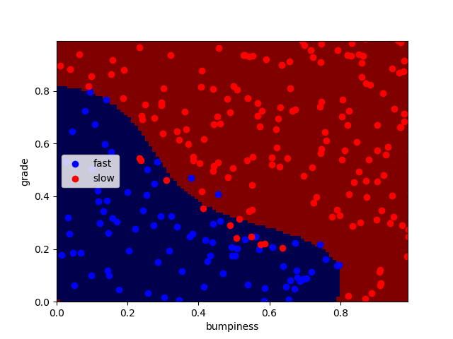
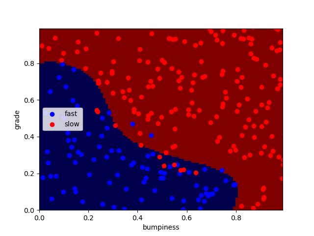
正确率分别为：92.4%　　 93.2%　　 94.4%

同时编译时间略微变长

有时训练集过大会使训练时间非常长，此时我们可以通过缩小训练集的方式来加快训练速度。
在训练分类器前加上这两句代码，可使训练集变为原本的1%：

features_train = features_train[:len(features_train)/100] 
labels_train = labels_train[:len(labels_train)/100]

SVM的优缺点

支持向量机在具有复杂领域和明显分割边界的情况下，表现十分出色。
但是，在海量数据集中，他的表现不太好，因为在这种规模的数据集中，训练时间将是立方数。（速度慢）
另外，在噪音过多的情况下，效果也不太好。（可能会导致过拟合）

posted @ 2019-02-24 01:31 Joeric 阅读(872) 评论(0) 编辑收藏举报

会员力量，点亮园子希望

刷新页面返回顶部

Joeric

支持向量机（SVM）

公告