ML—随机森林·1

Introduction to Random forest（Simplified）

With increase in computational power, we can now choose algorithms which perform very intensive calculations. One such algorithm is “Random Forest”, which we will discuss in this article. While the algorithm is very popular in various competitions (e.g. like the ones running on Kaggle), the end output of the model is like a black box and hence should be used judiciously（明智而审慎地）.

Before going any further, here is an example on the importance of choosing the best algorithm.

Importance of choosing the right algorithm

# 以作者看过的一部电影<明日边缘>引入：说明什么样的算法才是最佳算法？【红色高亮部分比喻很贴切】

Yesterday, I saw a movie called ” Edge of tomorrow“.  I loved the concept and the thought process which went behind the plot of this movie. Let me summarize the plot (without commenting on the climax, of course). Unlike other sci-fi movies, this movie revolves around one single power which is given to both the sides (hero and villain). The power being the ability to reset the day.

Human race is at war with an alien specie called “Mimics”.  Mimic is described as a far more evolved civilization of an alien specie. Entire Mimic civilization is like a single complete organism. It has a central brain called “Omega” which commands all other organisms in the civilization. It stays in contact with all other species of the civilization every single second. “Alpha” is the main warrior specie (like the nervous system) of this civilization and takes command from “Omega”. “Omega” has the power to reset the day at any point of time.

Now, let’s wear the hat of a predictive analyst to analyze this plot. If a system has the ability to reset the day at any point of time, it will use this power, whenever any of its warrior specie die. And, hence there will be no single war ,when any of the warrior specie (alpha) will actually die, and the brain “Omega” will repeatedly test the best case scenario to 【maximize the death of human race and put a constraint on number of deaths of alpha (warrior specie) to be zero】every single day. You can imagine this as “THE BEST” predictive algorithm ever made. It is literally impossible to defeat such an algorithm.

Let’s now get back to “Random Forests” using a case study.

Case Study

Following is a distribution of Annual income Gini Coefficients（基尼系数：高的基尼系数意味着该国的贫富差距相差很大） across different countries ：

Mexico has the second highest Gini coefficient and hence has a very high segregation in annual income of rich and poor. Our task is to come up with an accurate predictive algorithm to estimate annual income bracket（年收入档次） of each individual in Mexico. The brackets of income are as follows :

1. Below $40,000

2. $40,000 – 150,000

3. More than $150,000

Following are the information available for each individual ：

1. Age , 2. Gender,  3. Highest educational qualification, 4. Working in Industry, 5. Residence in Metro/Non-metro

We need to come up with an algorithm to give an accurate prediction for an individual who has following traits:

1. Age : 35 years , 2, Gender : Male , 3. Highest Educational Qualification : Diploma holder, 4. Industry : Manufacturing, 5. Residence : Metro

我们的任务就是：利用某一个人的年龄、性别、教育情况、工作领域以及住宅地共5个字段来预测他的收入层次！

We will only talk about random forest to make this prediction in this article.

The algorithm of Random Forest

Random forest is like a bootstrapping algorithm with Decision tree (CART) model. Say, we have 1000 observation in the complete population with 10 variables（比如：一个总体有1000个观测，10个变量）. Random forest tries to build multiple CART model with different sample and different initial variables（随机森林会使用不同的样本和初始值来构建多个CART模型）. For instance, it will take a random sample of 100 observation and 5 randomly（注意：每次都是随机的） chosen initial variables to build a CART model. It will repeat the process (say) 10 times and then make a final prediction on each observation. Final prediction is a function of each prediction(最终的预测是每次预测的一个函数). This final prediction can simply be the mean of each prediction（最终预测最简单的形式就是每次预测的平均！）.

bootstrapping这个概念

所谓的Bootstrapping法就是利用有限的样本资料经由多次重复抽样，重新建立起足以代表母体样本分布之新样本。

对于一个采样，我们只能计算出某个统计量(例如均值)的一个取值，无法知道均值统计量的分布情况。但是通过自助法(自举法)我们可以模拟出均值统计量的近似分布。有了分布很多事情就可以做了（比如说有你推出的结果来进而推测实际总体的情况）。

bootstrapping方法的实现很简单，假设你抽取的样本大小为n：

在原样本中有放回的抽样，抽取n次。每抽一次形成一个新的样本，重复操作，形成很多新样本，通过这些样本就可以计算出样本的一个分布。新样本的数量多少合适呢？大概1000就差不多行了，如果计算成本很小，或者对精度要求比较高，就增加新样本的数量。

最后这种方法的准确性和什么有关呢？这个我还不是清楚，猜测是和原样本的大小n，和Bootstrapping产生的新样本的数量有关系，越大的话越是精确，更详细的就不清楚了，想知道话做个搞几个已知的分布做做实验应该就清楚了。

Back to Case study

Disclaimer(免责声明) : The numbers in this article are illustrative（说明：本文中使用的数值都是虚构的）

Mexico has a population of 118 MM. Say, the algorithm Random forest picks up 10k observation with only one variable (for simplicity) to build each CART model（为了简化说明，规定随机森林每次选择1万条观测值和一个变量）. In total, we are looking at 5 CART model being built with different variables（看一看使用不同变量构建的5个CART模型！）. In a real life problem, you will have more number of population sample and different combinations of  input variables.

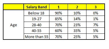
Salary bands :

Band 1 : Below $40,000

Band 2: $40,000 – 150,000

Band 3: More than $150,000

Following are the outputs of the 5 different CART model

CART 1 : Variable Age

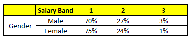
CART 2 : Variable Gender

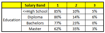
CART 3 : Variable Education

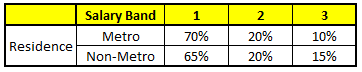
CART 4 : Variable Residence

CART 5 : Variable Industry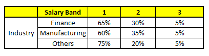

Using these 5 CART models, we need to come up with singe set of probability to belong to each of the salary classes（需要找到属于每一个工资类别的概率组合，为了简化，这里使用概率的平均作为一个指标）. For simplicity, we will just take a mean of probabilities in this case study. Other than simple mean, we also consider vote method（同时，还考虑了投票机制！） to come up with the final prediction. To come up with the final prediction let’s locate the following profile(概况：其实就是重温一下上面提到过的几个变量)n each CART model :

# 下面是一个观测值（即一个人）

1. Age : 35 years , 2, Gender : Male , 3. Highest Educational Qualification : Diploma holder, 4. Industry : Manufacturing, 5. Residence : Metro（这5五个变量相当于新的输入变量，通过这5个变量，我们需要预测他的工资层次）

For each of these CART model, following is the distribution across salary bands：(下面是各工资层次的分布)

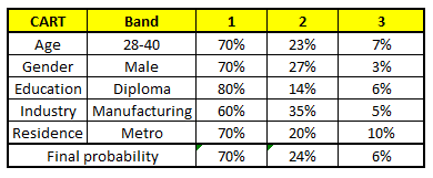
注：上面这个表是针对新输入变量的工资层次针对每个变量的概率分布以及通过平均单个变量的概率得到的最终概率！ so  cool！

The final probability is simply the average of the probability in the same salary bands in different CART models. As you can see from this analysis, that there is 70% chance of this individual falling in class 1 (less than $40,000) and around 24% chance of the individual falling in class 2.（最后，可以看到：这个人有70%的概率属于类别1，即工资收入低于40,000$）

End Notes

Random forest gives much more accurate predictions when compared to simple CART/CHAID or regression models in many scenarios(随机森林相比于简单CART或CHAID或回归模型预测精度更高！). These cases generally have high number of predictive variables and huge sample size（一般当预测变量比较多且样本比较大时运用随机森林的效果非常好！）. This is because it captures the variance of several input variables at the same time and enables high number of observations to participate in the prediction. In some of the coming articles, we will talk more about the algorithm in more detail and talk about how to build a simple random forest on R.

---

Comparing a CART model to Random Forest (Part 1)

I created my first simple regression model with my father in 8th standard (year: 2002) on MS Excel. Obviously, my contribution in that model was minimal, but I really enjoyed the graphical representation of the data. We tried validating all the assumptions etc. for this model. By the end of the exercise, we had 5 sheets of the simple regression model on 700 data points. The entire exercise was complex enough to confuse any person with average IQ level(看来作者的智商略高啊！！！). When I look at my models today, which are built on millions of observations and utilize complex statistics behind the scene, I realize how machine learning with sophisticated tools (like SAS, SPSS, R)  has made our life easy.

Having said that, many people in the industry do not bother about（置于不顾：我很在意啊，哈哈！）the complex statistics, which goes behind the scene. It becomes very important to realize the predictive power of each technique. No model is perfect in all scenarios（任何模型都不可能在所有的场景中达到效果最佳）. Hence, we need to understand the data and the surrounding eco-system before coming up with a model recommendation（因此，在构建一个之前，需要了解数据，以及围绕着数据的生态系统！作者的建议也正是我所推崇的啊！）。

In this article, we will compare two widely used techniques i.e. CART vs. Random forest. Basics of Random forest were covered in my last article. We will take a case study to build a strong foundation of this concept and use R to do the comparison. The dataset used in this article is an inbuilt dataset of R.

As the concept is pretty lengthy（要理解其中的概念确实需要细细品味，所以作者将其分成了两部分来讲！）, we have broken down this article into two parts！

Background on Dataset “Iris”

Data set “iris” gives the measurements in centimeters of the variables : sepal length and width and petal length and width, respectively, for 50 flowers from each of 3 species of Iris. The dataset has 150 cases (rows) and 5 variables (columns) named Sepal.Length, Sepal.Width, Petal.Length, Petal.Width, Species.（5个变量，其中使用前四个变量来预测花的种类） We intend to predict the Specie based on the 4 flower characteristic variables.

We will first load the dataset into R and then look at some of the key statistics. You can use the following codes to do so.

data(iris)

#look at the dataset

summary(iris)

#visually look at the dataset

qplot(Petal.Length,Petal.Width,colour=Species,data=iris)

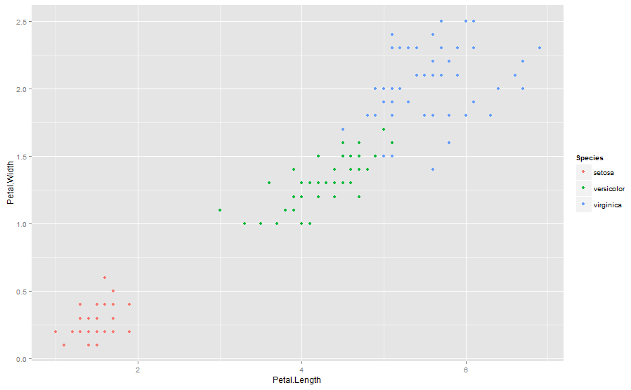
The three species seem to be well segregated from each other（可见，这三种花似乎彼此隔离的）. The accuracy in prediction of borderline cases determines the predictive power of the model（预测临界情形的精度决定了模型的预测能力）. In this case, we will install two useful packages for making a CART model.

library(rpart) #

library(caret) #

After loading the library, we will divide the population in two sets: Training and validation(将数据集分成两部分：训练集和校验集，各自占50%，这么做的目的是避免造成模型过拟合问题！). We do this to make sure that we do not overfit the model. In this case, we use a split of 50-50 for training and validation.

Generally, we keep training heavier to make sure that we capture the key characteristics（这个是常用的做法） You can use the following code to make this split.

train.flag <- 

createDataPartition

(y=iris$Species,p=0.5,list=FALSE)#这个函数用得好

training <- iris[train.flag,]

Validation <- iris[-train.flag,]

Building a CART model

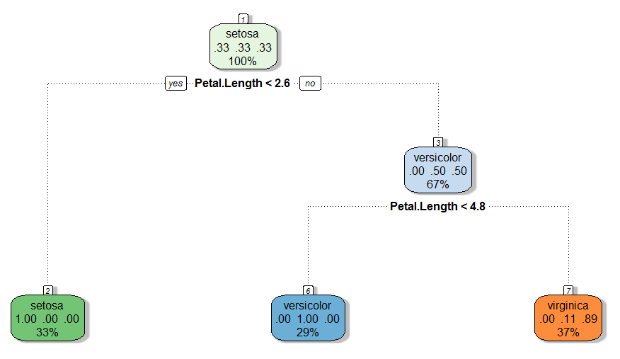
Once we have the two data sets and have got a basic understanding of data, we now build a CART model. We have used “caret” and “rpart” package to build this model. However, the traditional representation of the CART model is not graphically appealing on R. Hence, we have used a package called “rattle” to make this decision tree. “Rattle” builds a more fancy and clean trees, which can be easily interpreted. Use the following code to build a tree and graphically check this tree（使用了三个包来构建CART模型：caret、rpart和rattle包）：

modfit <- train(Species~.,method="rpart",data=training) 

library(rattle)

fancyRpartPlot(modfit$finalModel)

Validating the model

Now, we need to check the predictive power of the CART model, we just built. Here, we are looking at a discordance rate (which is the number of misclassifications in the tree：这里所说的discordance rate，直译是不一致率，其实指的是模型树的错分数量，一般用这个指标作为决策的标准！) as the decision criteria. We use the following code to do the same :

train.cart<-predict(modfit,newdata=training)

table(train.cart,training$Species)

train.cart   setosa versicolor virginica

---

setosa         25         0          0

versicolor     0         22         0

virginica       0         3         25

# 

Misclassification rate

 = 3/75（得到错分率！！！）

Only 3 misclassified observations out of 75, signifies good predictive power（可以看到，针对75个观测的预测只出现了3次错误分类，说明模型预测能力还是可以！）. In general, a model with misclassification rate less than 30% is considered to be a good model（一般情况下，错分率小于30%的模型被认为是一个良好的模型，但是一个好模型的判别范围还取决于不同的产业和问题的本质！）. But, the range of a good model depends on the industry and the nature of the problem. Once we have built the model, we will validate the same on a separate data set. This is done to make sure that we are not over fitting the model. In case we do over fit the model, validation will show a sharp decline in the predictive power. It is also recommended to do an out of time validation of the model. This will make sure that our model is not time dependent. For instance, a model built in festive time, might not hold in regular time. For simplicity, we will only do an in-time validation of the model. We use the following code to do an in-time validation（模型校验，这里使用及时校验方法，必要的时候建议使用out of time validation方法，这样可以避免我们的模型不会依赖于时间，比如在万圣节数据生成的模型可能不会再常规时间下适用啊！）:

pred.cart<-predict(modfit,newdata=Validation)

table(pred.cart,Validation$Species)

---

pred.cart   setosa    versicolor virginica

setosa         25         0         0

versicolor     0         22        1

virginica       0         3        24

# Misclassification rate = 4/75

As we see from the above calculations that the predictive power decreased in validation as compared to training（可以看到，模型对于校验数据的预测能力下降啦，这是很正常的！当校验集产生的错误率与训练集产生的错误率接近时，可以认为模型是比较稳定的！可以看到，我们取得的CART模型是比较稳定的,nice啊！）. This is generally true in most cases. The reason being, the model is trained on the training data set, and just overlaid on validation training set. But, it hardly matters, if the predictive power of validation is lesser or better than training. What we need to check is that they are close enough. In this case, we do see the misclassification rate to be really close to each other. Hence, we see a stable CART model in this case study.

Let’s now try to visualize the cases for which the prediction went wrong（可视化一下那些引起错误分类的观测）. Following is the code we use to find the same :

correct <- pred.cart == Validation$Species

qplot(Petal.Length,Petal.Width,colour=correct,data=Validation)

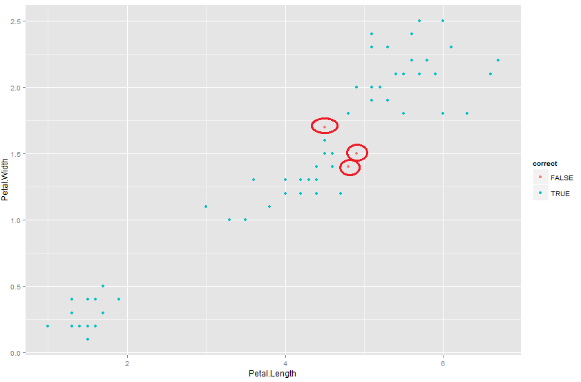
As you see from the graph, the predictions which went wrong were actually those borderline cases(可以看到，引起错分的观测都是位于类与类之间的临界点). We have already discussed before that these are the cases which make or break the comparison for the model. Most of the models will be able to categorize observation far away from each other. It takes a model to be sharp to distinguish these borderline cases.

End Notes :

In the next article, we will solve the same problem using a random forest algorithm（下节预告：下一部分将会讨论随机森林，我们可以得知：随机森林能够很好的处理这些由于临界值引起的问题！）. We hope that random forest will be able to make even better prediction for these borderline cases. But, we can never generalize the order of predictive power among a CART and a random forest, or rather any predictive algorithm. The reason being every model has its own strength. Random forest generally tends to have a very high accuracy on the training population, because it uses many different characteristics to make a prediction. But, because of the same reason, it sometimes over fits the model on the data. We will see these observations graphically in the next article and talk in more details on scenarios where random forest or CART comes out to be a better predictive model.

Comparing a Random Forest to a CART model (Part 3)

Random forest is one of the most commonly used algorithm in Kaggle competitions. Along with a good predictive power, Random forest model are pretty simple to build. We have previously explained the algorithm of a random forest ( Introduction to Random Forest ). This article is the second part of the series on comparison of a random forest with a CART model. In the first article, we took an example of an inbuilt R-dataset to predict the classification of an specie. In this article we will build a random forest model on the same dataset to compare the performance with previously built CART model（该节将对相同的数据集构建一个随机模型，从而与之前构建的CART模型进行性能对比）. I did this experiment a week back and found the results very insightful. I recommend the reader to read the first part of this article (Last article) before reading this one.

Background on Dataset “Iris”

Data set “iris” gives the measurements in centimeters of the variables : sepal length and width and petal length and width, respectively, for 50 flowers from each of 3 species of Iris. The dataset has 150 cases (rows) and 5 variables (columns) named Sepal.Length, Sepal.Width, Petal.Length, Petal.Width, Species. We intend to predict the Specie based on the 4 flower characteristic variables(再次熟悉了一下数据集，并且说明了预测任务：基于花的4个特征变量来预测花的种类).

We will first load the dataset into R and then look at some of the key statistics. You can use the following codes to do so.

data(iris)

# look at the dataset

summary(iris)

# visually look at the dataset

qplot(Petal.Length,Petal.Width,colour=Species,data=iris)

Results using CART Model

The first step we follow in any modeling exercise is to split the data into training and validation. You can use the following code for the split. (We will use the same split for random forest as well)

注：这里用来分隔数据的方法和之前的CART模型一样！

train.flag <- createDataPartition(y=iris$Species,p=0.5,list=FALSE)

training <- iris[train.flag,]

Validation <- iris[-train.flag,]

CART model gave following result in the training and validation :

Misclassification rate in training data = 3/75  #训练集的错分率是3/75

Misclassification rate in validation data = 4/75 #校验集中的错分率是4/75

As you can see, CART model gave decent result in terms of accuracy and stability. We will now model the random forest algorithm on the same training dataset and validate it using same validation dataset.

Building  a Random forest model

We have used “caret” , “randomForest” and “randomForestSRC” （使用caret、randomForest、randomForestSRC三个包来构建随机森林模型！）package to build this model. You can use the following code to generate a random forest model on the training dataset。

> library(randomForest)

> library(randomForestSRC)

> library(caret)

> modfit <- train(Species~ .,method="rf",data=training)

> train.RF<- predict(modfit,training)

> table(train.RF,training$Species)

---

 pred       setosa versicolor virginica
 setosa        25       0          0
 versicolor     0      25          0
 virginica      0       0         25

Misclassification rate in training data = 0/75 [This is simply awesome!]（错分率居然为0）

Validating the model

Having built such an accurate model, we will like to make sure that we are not over fitting the model on the training data. This is done by validating the same model on an independent data set. We use the following code to do the same :

> Pred.RF<-predict(modfit,newdata=Validation)

> table(Pred.RF,Validation$Species)

---

Pred.RF      setosa versicolor virginica
 setosa        25       0          0
 versicolor     0      22          0
 virginica      0       3         25

 # Misclassification rate = 3/75

Only 3 misclassified observations out of 75, signifies good predictive power. However, we see a significant drop in predictive power of this model when we compare it to training misclassification.（可以看到，75个观测值中，只有3个预测错误，显示模型预测能力还可以！同时：对比CART模型的错分率结果，我们发现随机森林模型的预测能力较高！）

Comparison between the two models

Till this point, everything was as per（按照，依据；如同） books. Here comes the tricky part. Once you have all performance metrics, you need to select the best model as per your business requirement. We will make this judgement based on 3 criterion（提出选择模型的三个标准） in this case apart from business requirements:

.1. Stability（稳定性） : The model should have similar performance metrics across both training and validation. This is very essential because business can live with a lower accuracy but not with a lower stability. We will give the highest weight to stability. For this case let’s take it as 5（在商业运用中，稳定性通常是最重要的，这里给稳定性的权重赋值为5）.

2. Performance on Training data（训练集上的性能表现） : This is one of the important metric but nothing conclusive can be said just based on this metric. This is because an over fit model is unacceptable but will get a very high score at this parameter. Hence, we will give a low weight to this parameter (say 2)（训练集上的性能表现赋值为2）.

3. Performance on Validation data : This metric catch holds of overfit model and hence is an important metric. We will score it higher than performance and lower than stability. For this case let’s take it as 3（校验集上的表现赋值为3）.

Note that the weights and scores entirely depends on the business case. Following is a score table as per my judgement in this case（最终根据以上三个指标及相应权重得到一个模型打分表）。

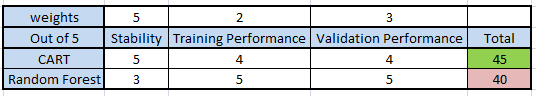
有一个问题：这个打分表针对CART模型和Random Forest模型的稳定性、训练集性能表现、校验集性能表现的得分是怎么得到的呢？是直接主观打分呢，还是根据一定的概率算出来的呢？[我觉得这里作者应该是直接进行的主观打分！有意见的朋友欢迎提出来哈，共同进步，oh yeah！]

===================================================================================

As you can see from the table that however Random forest gives me a better performance, I still will go ahead and use CART model because of the stability factor（结论：可以看到，尽管随机森林的性能更高，但是我们仍然会选择CART模型，因为CART模型的稳定性因素更高）. Other factor in favor of CART model is the easy business justification. Random forest is very difficult to explain to people working on field. CART models are simple cuts which can be justified by simple business justification/reasons. But the choice of model selection is entirely dependent on business requirement（不管怎么说，模型的选择完全取决于商业需求！）.

End Notes

Every model has its own strength. Random forest, as seen from this case study, has a very high accuracy on the training population, because it uses many different characteristics to make a prediction. But, because of the same reason, it sometimes over fits the model on the data. CART model on the other side is simplistic criterion cut model. This might be over simplification in some case but works pretty well in most business scenarios. However, the choice of model might be business requirement dependent, it is always good to compare performance of different model before taking this call（最后阐释了一下Random Forest和CART的优劣势，并对模型的选择给出了温馨提示：模型的选择依赖于具体的商业需求！！！）.

Entire scripts summarized
1）CART模型	2）Random Forest
#加载iris数据集并查看数据特征 data(iris) # look at the dataset summary(iris) # visually look at the dataset qplot(Petal.Length,Petal.Width, colour=Species,data=iris) #加载rpart和caret包 library(rpart) library(caret) # 构造训练集和校验集 train.flag <- createDataPartition #[来自caret包] (y=iris$Species,p=0.5,list=FALSE) training <- iris[train.flag,] Validation <- iris[-train.flag,] # 构建CART模型 modfit <- train (Species~.,method="rpart",data=training) library(rattle)# 加载rattle是为了产生更美观的决策树 fancyRpartPlot(modfit$finalModel) # 使用训练集和校验集验证模型！ train.cart<-predict(modfit,newdata= training ) table(train.cart,training$Species) #Results：Misclassification rate = 3/75 pred.cart<-predict(modfit,newdata= Validation ) table(pred.cart,Validation$Species) #Results：Misclassification rate = 4/75#可视化观测值，检测出时哪些观测值导致错分 correct <- pred.cart == Validation$Species qplot(Petal.Length,Petal.Width,colour=correct,data=Validation)	#加载iris数据集并查看数据特征 data(iris) # look at the dataset summary(iris) # visually look at the dataset qplot(Petal.Length,Petal.Width, colour=Species,data=iris) # 构造训练集和校验集 train.flag <- createDataPartition(y=iris$Species,p=0.5,list=FALSE) training <- iris[train.flag,] Validation <- iris[-train.flag,] #加载caret , randomForest和randomForestSRC三个包 > library(randomForest) > library(randomForestSRC) > library(caret) # 构建RF模型 > modfit <- train(Species~ .,method="rf",data=training) # 使用训练集和校验集验证模型 > train.RF <- predict(modfit,training) > table(train.RF,training$Species) #Results：Misclassification rate in training data = 0/75    > pred.RF<-predict(modfit,newdata=Validation) > table(pred.RF,Validation$Species) #Results：Misclassification rate = 3/75

暂时没理解的部分[模型打分的根据是什么？]

参考文献

http://www.analyticsvidhya.com/blog/2014/06/comparing-random-forest-simple-cart-model/（Part1）

http://www.analyticsvidhya.com/blog/2014/06/comparing-random-forest-simple-cart-model/（Part2）

我的代码实践

#Step1：先把所需要的包都一并加载啦！

> require(ggplot2) #要使用该包中的qplot画图
> require(caret) 

> require(rpart)

> require(rattle) #该包中的fancyRpartPlot函数可以绘制更美观的决策树！

> require(randomForest)

> require(randomForestSRC)

#Step2：加载iris案例数据集并查看数据特征

> data(iris)
> 

summary

(iris)

 Sepal.Length    Sepal.Width     Petal.Length    Petal.Width          Species  
 Min.   :4.300   Min.   :2.000   Min.   :1.000   Min.   :0.100   setosa    :50  
 1st Qu.:5.100   1st Qu.:2.800   1st Qu.:1.600   1st Qu.:0.300   versicolor:50  
 Median :5.800   Median :3.000   Median :4.350   Median :1.300   virginica :50  
 Mean   :5.843   Mean   :3.057   Mean   :3.758   Mean   :1.199                  
 3rd Qu.:6.400   3rd Qu.:3.300   3rd Qu.:5.100   3rd Qu.:1.800                  
 Max.   :7.900   Max.   :4.400   Max.   :6.900   Max.   :2.500  

>qplot(Petal.Length,Petal.Width,colour=Species,data=iris,shape=Species,color=Species)

#Step3：构造训练集和验证集

> train.flag <- createDataPartition (y=iris$Species,p=0.5,list=FALSE)

#p表示提取到训练集中的百分比数据;y表示结果变量组成的向量.

#createDataPartition函数是caret包中用于拆分数据的函数之一，其系列家族函数的用法会在另一篇文章中介绍！
> training <- iris[train.flag,]
> Validation <- iris[-train.flag,]

> head(iris)
  Sepal.Length Sepal.Width Petal.Length Petal.Width Species
1          5.1         3.5          1.4         0.2  setosa
2          4.9         3.0          1.4         0.2  setosa
3          4.7         3.2          1.3         0.2  setosa
4          4.6         3.1          1.5         0.2  setosa
5          5.0         3.6          1.4         0.2  setosa
6          5.4         3.9          1.7         0.4  setosa
> head(train.flag)
     Resample1
[1,]         1
[2,]         3
[3,]         4
[4,]         5
[5,]         6
[6,]         7
> head(training)
  Sepal.Length Sepal.Width Petal.Length Petal.Width Species
1          5.1         3.5          1.4         0.2  setosa
3          4.7         3.2          1.3         0.2  setosa
4          4.6         3.1          1.5         0.2  setosa
5          5.0         3.6          1.4         0.2  setosa
6          5.4         3.9          1.7         0.4  setosa
7          4.6         3.4          1.4         0.3  setosa
> head(Validation)
   Sepal.Length Sepal.Width Petal.Length Petal.Width Species
2           4.9         3.0          1.4         0.2  setosa
10          4.9         3.1          1.5         0.1  setosa
15          5.8         4.0          1.2         0.2  setosa
16          5.7         4.4          1.5         0.4  setosa
19          5.7         3.8          1.7         0.3  setosa
21          5.4         3.4          1.7         0.2  setosa

备注：可知，createDataPartition 拆分数据是随机进行的！

#Step4：构建CART模型，并可视化结果决策树

> modfit <- 

train

(Species~.,method="rpart",data=training)#train来自caret包,用法参见另一篇文章

### train方法返回一个模型对象,该对象中包含了以下方法（重要的方法用红色高亮）

method	建模方法	modfit$method: " rpart
modelInfo	模型对象信息	包含以下函数：grid+loop+fit+predict+prob+predictors+varImp
modelType	模型类型	modfit$modelType： Classification
results	拟合结果	cp Accuracy Kappa AccuracySD KappaSD 1 0.00 0.9418214 0.9105524 0.05087244 0.0808062 2 0.48 0.6461598 0.4827485 0.17475020 0.2376012 3 0.50 0.5393118 0.3349623 0.13902303 0.1651445
pred		modfit$pred:NULL
bestTune	得到的cp最佳参数	modfit$bestTune: cp[0]
call	训练模型调用的函数	train.formula(form=Species ~. , data = training, method = "rpart")
dots		list()
metric	评估模型好坏的指标	modfit$metric：" Accuracy ”
control	具体采用的CART方法及每次抽样数据	比如：$method： "boot"；$repeats：25；$p：0.75； $index（保存每次重复抽样数据的索引）;$indexout(保存了未被抽样数据的索引)
finalModel	最终的模型	简单分类树的结构（结合fancyRpartPlot函数绘制决策树图形）
preProcess	预处理	NULL
trainingData	用来训练模型的数据	你懂的！
resample	每次重复抽样计算得到的精确度！	Accuracy Kappa Resample 1 0.9032258 0.8514377 Resample09 2 0.8888889 0.8272921 Resample05 ……………………此处省略………………… 24 0.9642857 0.9459459 Resample21 25 0.9677419 0.9514107 Resample17
resampledCM		cp cell1 cell2 cell3 cell4 cell5 cell6 cell7 cell8 cell9 Resample 1 0.00 7 0 0 0 7 3 0 0 13 Resample01 2 0.44 7 0 0 0 10 0 0 13 0 Resample01………………………………………省略……………………………………….…74 0.44 7 0 0 0 8 0 0 8 0 Resample25 75 0.50 7 0 0 0 8 0 0 8 0 Resample25
perfNames	performanceNames	modfit$perfNames ："Accuracy" "Kappa"
maximize		modfit$maximize：TRUE
yLimits		NULL
times	记录模型训练所用时间	$everything 用户 系统 流逝 1.01 0.03 1.05
terms
coefnames		预测变量：Sepal.Length, Sepal.Width, Petal.Length, Petal.Width
xlevels

> 

fancyRpartPlot

(modfit$

finalModel

) #该函数来自rattle包,用于绘制美观的RPart决策树（注意：海里还需要加载rpart.plot包）

# Step5：模型校验

#1)利用训练数据的预测变量来预测Species 

> train.cart<-

predict

(modfit,newdata=training

>train.cart（预测值）

[1] setosa setosa setosa setosa setosa setosa setosa [8] setosa setosa setosa setosa setosa setosa setosa [15] setosa setosa setosa setosa setosa setosa setosa [22] setosa setosa setosa setosa versicolor versicolor versicolor [29] versicolor versicolor versicolor versicolor versicolor versicolor versicolor [36] versicolor versicolor versicolor versicolor versicolor versicolor versicolor [43] virginica versicolor versicolor versicolor versicolor versicolor versicolor [50] versicolor virginica virginica virginica virginica versicolor virginica [57] virginica virginica virginica virginica virginica versicolor virginica [64] virginica virginica virginica virginica virginica virginica virginica [71] virginica virginica virginica virginica virginica Levels: setosa versicolor virginica

---

> training$Species（原始值）

[1] setosa setosa setosa setosa setosa setosa setosa [8] setosa setosa setosa setosa setosa setosa setosa [15] setosa setosa setosa setosa setosa setosa setosa [22] setosa setosa setosa setosa versicolor versicolor versicolor [29] versicolor versicolor versicolor versicolor versicolor versicolor versicolor [36] versicolor versicolor versicolor versicolor versicolor versicolor versicolor [43] versicolor versicolor versicolor versicolor versicolor versicolor versicolor [50] versicolor virginica virginica virginica virginica virginica virginica [57] virginica virginica virginica virginica virginica virginica virginica [64] virginica virginica virginica virginica virginica virginica virginica [71] virginica virginica virginica virginica virginica Levels: setosa versicolor virginica预测值与原始值对比，甄别出预测值中预测错误的点（用红色高亮的地方！）

> 

table

(train.cart,training$Species)

train.cart setosa versicolor virginica
setosa       25       0         0
versicolor   0        24        2
virginica    0        1         23
# 列表示预测类别，行表示原始类别.
# 可见:本来是virginica的有2个被预测成了versicolor,versicolor有一个被预测成了virginica
所以可以得到错分率=(2+1)/(25+25+25)=3/75

#2))#利用验证集的预测变量来预测Species

> pred.cart<-predict(modfit,newdata=Validation)
> table(pred.cart,Validation$Species)

pred.cart    setosa versicolor virginica
  setosa         25          0         0
  versicolor      0         25         7
  virginica       0          0        18

#同理可得：有7次预测错误, 错分率=7/75

# Step6：可视化观测值，检测出时哪些观测值导致错分

> correct <- pred.cart == Validation$Species

[1] TRUE TRUE TRUE TRUE TRUE TRUE TRUE TRUE TRUE TRUE TRUE TRUE TRUE TRUE [15] TRUE TRUE TRUE TRUE TRUE TRUE TRUE TRUE TRUE TRUE TRUE TRUE TRUE TRUE [29] TRUE TRUE TRUE TRUE TRUE TRUE TRUE TRUE TRUE TRUE TRUE TRUE TRUE TRUE [43] TRUE TRUE TRUE TRUE TRUE TRUE TRUE TRUE TRUE TRUE TRUE TRUE TRUE TRUE [57] FALSE TRUE FALSE TRUE FALSE TRUE TRUE FALSE FALSE TRUE TRUE TRUE TRUE FALSE [71] TRUE TRUE TRUE FALSE TRUE

> qplot(Petal.Length,Petal.Width,colour=correct,data=Validation)

---

# Step7：构建RF模型

> modfit <- train(Species~ .,method="rf",data=training) #得到modfit模型对象中的方法和CART一样！

#

Step8: 模型校验

> pred <- predict(modfit,training)

> pred [1] setosa setosa setosa setosa setosa setosa setosa [8] setosa setosa setosa setosa setosa setosa setosa [15] setosa setosa setosa setosa setosa setosa setosa [22] setosa setosa setosa setosa versicolor versicolor versicolor [29] versicolor versicolor versicolor versicolor versicolor versicolor versicolor [36] versicolor versicolor versicolor versicolor versicolor versicolor versicolor [43] versicolor versicolor versicolor versicolor versicolor versicolor versicolor [50] versicolor virginica virginica virginica virginica virginica virginica [57] virginica virginica virginica virginica virginica virginica virginica [64] virginica virginica virginica virginica virginica virginica virginica [71] virginica virginica virginica virginica virginica Levels: setosa versicolor virginica > training$Species [1] setosa setosa setosa setosa setosa setosa setosa [8] setosa setosa setosa setosa setosa setosa setosa [15] setosa setosa setosa setosa setosa setosa setosa [22] setosa setosa setosa setosa versicolor versicolor versicolor [29] versicolor versicolor versicolor versicolor versicolor versicolor versicolor [36] versicolor versicolor versicolor versicolor versicolor versicolor versicolor [43] versicolor versicolor versicolor versicolor versicolor versicolor versicolor [50] versicolor virginica virginica virginica virginica virginica virginica [57] virginica virginica virginica virginica virginica virginica virginica [64] virginica virginica virginica virginica virginica virginica virginica [71] virginica virginica virginica virginica virginica Levels: setosa versicolor virginica# 哇啊，居然是0错误！碉堡了！

> table(train.cart,training$Species)

pred         setosa versicolor virginica
  setosa         25          0         0
  versicolor      0         25         0
  virginica       0          0        25

> train.RF<-predict(modfit,newdata=Validation)
> table(train.RF,Validation$Species)

train.RF     setosa versicolor virginica
  setosa         25          0         0
  versicolor      0         25         3
  virginica       0          0        22

# 错误率=3/75

# Step9：可视化观测值，检测出时哪些观测值导致错分

> correct <- train.RF == Validation$Species
> qplot(Petal.Length,Petal.Width,colour=correct,data=Validation)

---