预测美国债券回报

目录

• Forecasting US Bond Returns
  • INTRODUCTION
  • REASON FOR THE CHANGING RISK PREMIUM: A CYCLE OF FEAR AND GREED
  • ARE EXCESS BOND RETURNS PREDICTABLE?
    • Correlations Between Predictor Variables and Subsequent Excess Bond Return
    • Out-of-Sample Estimation of Return Predictions
  • INVESTMENT IMPLICATIONS OF BOND RETURN PREDICTABILITY
    • Exploiting Return Predictability by Using Dynamic Investment Strategies
    • Stability of the Predictive Relations
    • Other Critical Considerations
    • Impact of Investment Horizon
  • CONCLUDING REMARKS
  • LITERATURE GUIDE

著：Antti Ilmanen 译：徐瑞龙

Forecasting US Bond Returns

预测美国债券回报

INTRODUCTION

引言

It is extremely difficult to forecast bond market fluctuations. However, recent research shows that these fluctuations are not fully unpredictable: It is possible to identify in advance periods when the reward for duration extension is likely to be abnormally high or abnormally low. In this report, we first describe a few variables that have the ability to predict near-term bond market performance. We then show how to combine the information that these predictors contain into a single forecast and, further, into implementable investment strategies. Finally, we backtest the historical performance of these strategies in a realistic "out-of-sample" setting.

预测债券市场的变动是非常困难的。然而，最近的研究表明，这些变动并不是完全不可预测的：有可能提前确定增加久期是否会使回报异常高或异常低。在本报告中，我们首先描述一些能够预测近期债券市场表现的变量。然后，我们将展示如何将这些预测变量所包含的信息组合成单一预测，并成为可实施的投资策略。最后，我们以现实的“样本外”数据来回顾这些策略的历史表现。

This report is the fourth part of a series titled Understanding the Yield Curve. Historical analysis included in Part 3, Does Duration Extension Enhance Long-Term Expected Returns?, showed that intermediate- and long-term bonds earn higher average returns than short-term bonds. This evidence suggests that the long-run bond risk premium is positive.^[1] If the risk premium is constant over time, the long-run average risk premium is also our best forecast for the near-term bond market performance. However, we showed in Part 3 that steeply upward-sloping yield curves tend to precede high excess bond returns and inverted yield curves tend to precede negative excess bond returns. It follows then that the risk premium is not constant and that the current shape of the yield curve provides valuable information about the time-varying bond risk premium. In this report, we show that other variables can enhance the yield curve's ability to forecast the near-term excess bond return. The predictability of the excess bond return has important implications for investors who are willing to use so-called tactical asset allocation strategies. Based on our extensive historical analysis, strategies that adjust the portfolio duration dynamically using the signals from the predictor variables would have earned substantially higher long-run returns than did static strategies that do not actively adjust the portfolio duration.

本报告是《理解收益率曲线》系列的第四部分。历史分析包括在第三部分（《久期增加会提高长期预期回报吗？》）中，分析表明中期和长期债券的平均回报高于短期债券。这个证据表明长期债券的风险溢价是正的。如果风险溢价随时间不变，长期平均风险溢价也是近期债券市场表现的最佳预测。然而，我们在第三部分中显示，陡峭的向上倾斜的收益率曲线倾向于预示高的债券超额回报，而倒挂的收益率曲线倾向于预示负的债券超额回报。因此，风险溢价不是恒定的，而目前的收益率曲线形状提供了（时变的）债券风险溢价的有用信息。在本报告中，我们指出某些变量可以提高收益率曲线预测近期债券超额回报的能力。债券超额回报的可预测性对于愿意使用所谓的战术资产配置策略的投资者而言具有重要意义。根据我们广泛的历史分析，使用预测变量的信号动态调整投资组合久期的策略将比没有积极调整投资组合久期的静态策略获得更高的长期回报。

REASON FOR THE CHANGING RISK PREMIUM: A CYCLE OF FEAR AND GREED

风险溢价变化的原因：恐惧与贪婪的循环

Earlier empirical research shows that the expected excess returns of stocks and long-term bonds vary over the business cycle: they tend to be high at the end of the recession and low at the end of the expansion. Are there any intuitive reasons that expected excess returns should vary with economic conditions?

早期的实证研究表明，股票和长期债券的预期超额回报随商业周期变化而有所不同：经济衰退结束时趋于高位，而在扩张结束时趋于低位。预期超额回报随经济条件而变化，这是否有直观的解释？

If the expected returns reflect rational risk premia, they change over time as the amount of risk in assets or the market price of risk varies over time. The risk premium that bond market participants expect should increase if the risk increases (because of higher interest rate volatility, higher covariance between bonds and stocks, greater inflation uncertainty, etc). In addition, the required risk premium should increase if the market participants' aggregate risk aversion level increases. We propose that investors are more risk averse (afraid) when their current wealth is low relative to their past wealth. The higher risk aversion makes them demand higher risk premia (larger compensation for holding risky assets) near business cycle troughs. Conversely, higher wealth near business cycle peaks makes investors less risk averse (more complacent and greedy); therefore, they bid down the required risk premia (by bidding up the asset prices). Thus, the observed time-variation in risk premia may be explained by the old Wall Street adage about the cycle of fear and greed.

如果预期回报反映出合理的风险溢价，则预期回报会像资产风险或风险的市场价格一样随时间而变化。如果风险增加（由于收益率波动率较大、债券和股票之间的协方差变高、通货膨胀的不确定性等），债券市场参与者预期的风险溢价将会增加。此外，如果市场参与者的总体风险规避水平提高，则所要求的风险溢价应增加。我们观察到投资者，当目前的财富低于过去的财富时更为倾向于风险厌恶（恐惧）。较高的风险厌恶程度使得他们在商业周期低谷附近要求更高的风险溢价（较高的持有风险资产的补偿）。相反，在商业周期高峰附近的更多的财富使投资者的风险厌恶偏低（更自满和贪婪）;因此，他们降低所要求的风险溢价（通过提高资产价格）。因此，观察到的风险溢价的时变性可能由华尔街上关于恐惧与贪婪循环的古老格言来解释的。

ARE EXCESS BOND RETURNS PREDICTABLE?

债券超额回报是可预测的？

Which Variables Forecast the Excess Bond Return?

哪些变量能预测债券超额回报？

As mentioned above, measures of yield curve steepness have some ability to predict the subsequent excess bond return. In the appendix to Part 2 of this series, Market's Rate Expectations and Forward Rates, we showed that a steep yield curve may reflect a high required risk premium or the market's expectations of rising rates. If the second term is assumed to be zero (the current yield curve is the market's best forecast for future yield curves), then the curve steepness is a good proxy for the bond risk premium. We measure the curve steepness by the term spread (the difference between a long-term rate and a short-term rate).

如上所述，收益率曲线的陡峭程度具有一定的预测后续债券超额回报的能力。在本系列第二部分（《市场收益率预期与远期收益率》）的附录中我们表明，陡峭的收益率曲线可能反映了高风险溢价或市场对收益率上涨的预期。如果第二项假设为零（即当前的收益率曲线是市场对未来收益率曲线的最佳预测），那么曲线陡峭程度是债券风险溢价的良好代表。我们通过期限利差（长期收益率和短期收益率之间的差额）来衡量曲线陡峭程度。

Conveniently, we can use the term spread as an overall proxy for the bond risk premium even if we do not know what causes the expected return differentials across bonds. For this reason, the term spread will be our first predictor variable. Yet, if we are trying to forecast bond returns, why restrict ourselves to just one predictor? It is likely that the term spread is sometimes influenced by the market's rate expectations, making the previous assumption unrealistic. Because the rate expectations are unobservable, we cannot know how much "noise" they introduce to our risk premium proxy. Thus, we do not know to what extent a given shape of the curve reflects the required bond risk premium and to what extent it reflects the market's rate expectations. Using other predictor variables together with the term spread should help us filter out the noise and give us a better signal about the future risk premium.

方便的是，即使我们不知道是什么原因导致债券的预期回报差异，我们也可以将期限利差用作债券风险溢价的总体代表。因此，期限利差将是我们的第一个预测变量。然而，如果我们试图预测债券回报，为什么只限制一个预测指标？期限利差有可能受到市场收益率预期的影响，使得以前的假设变得不切实际。由于收益率预期不可观察，我们无法知道风险溢价的代表被引入了多少“噪音”。因此，我们不知道曲线的特定形状在多大程度上反映了所要求的债券风险溢价，以及它在多大程度上反映了市场的收益率预期。综合使用其他预测变量与期限利差应该有助于我们消除噪音，并为未来的风险溢价提供更好的信号。

The filter variables should be correlated with the risk premium. Based on our hypothesis of wealth-dependent risk aversion, we combine the information in the term spread and in the stock market's recent performance. The inverse of the recent stock market performance is our proxy for the (unobservable) aggregate level of risk aversion. If a high term spread coincides with a depressed stock market, the curve steepness is less likely to reflect rising rate expectations (because monetary policy tightening and inflation threat are less likely in this environment) and more likely to reflect high required risk premia (because low stock prices may reflect high required returns on risky assets, or even cause them via wealth-dependent risk aversion). We measure the recent stock market performance by "inverse wealth," a weighted average of past returns, where more distant observations have lower weights.

过滤变量应与风险溢价相关。基于我们对财富依赖风险厌恶的假设，我们将期限利差中的信息和股票市场近期业绩相结合。近期股票表现的逆是我们对（不可观察的）风险厌恶总体水平的代表。如果高期限利差与股市萧条相吻合，那么曲线陡峭程度不太可能反映收益率上升预期（因为货币政策紧缩和通货膨胀威胁在这种环境中不大可能发生），更有可能反映出对高风险溢价的要求（因为处于低位的股票价格可能会反映风险资产所要求的高回报，或甚至通过财富依赖风险厌恶来引发）。我们通过“逆财富”衡量近期股市表现，这是过去回报的加权平均数，其中更久远的观察具有较低的权重。

As a third predictor, we will examine the real bond yield, which is sometimes used as the overall proxy for the bond risk premium instead of the term spread. This measure incorporates the inflation rate into the forecasting model. Our final predictor, momentum, is a dummy variable that simulates a simple moving average trading rule to exploit the persistence (positive autocorrelation) in bond returns.^[2] This strategy tries to capture large trending moves in the bond market. To reduce trading when the yields are oscillating within a narrow trading range and, thereby, to avoid "whipsaw" losses from buying at low yields and selling at high yields, we impose a neutral trading range in which no position is held. Somewhat arbitrarily, we use a six-month moving average window and a ten-basis-point neutral trading range. Thus, the rule is to take a long (short) position in the bond market when the long-term bond yield declines (increases) to more than five basis points below (above) its six-month moving average: such a break-out from a trading range is attributed to positive (negative) momentum in the bond market. If the bond yield returns to (stays within) the ten-basis-point range around its six-month average, the rule is to take (retain) a neutral position. The dummy variable takes value 1, -1 or 0 if the strategy is long, short or neutral, respectively.

作为第三个预测因素，我们将考察债券收益率，有时被用作债券风险溢价的整体代表，而不是期限利差。这一措施将通货膨胀率纳入预测模型。我们的最后一个预测因素是动量，它是一个虚拟变量，它遵从一个简单的移动平均交易规则来利用债券回报中的持续性（正的自相关）。这一策略试图在债券市场上捕捉大趋势。当收益率在狭窄的交易范围内波动时，为了减少交易，避免在低收益率购买和高收益率卖出的“鞭打”损失，我们强加了一个中性的交易范围，在这里没有任何仓位。我们有些主观地使用六个月的移动平均窗口和十个基点的中性交易范围。规则就是当长期债券收益率下降（上升）至六个月移动平均线以下超过五个基点以上时做多（做空）：从交易区间来看，这样一个突破表明债券市场呈正（负）趋势。如果债券收益率返回其六个月平均水平左右十个基点范围内，则该规则要求持仓不变。策略做多、做空或不变，相应的虚拟变量分别取值为1，-1或0。

Our empirical analysis will confirm that the term spread can forecast future excess bond returns, but combining the information contained in several predictor variables improves these forecasts further. Linear regression is the most common way to combine the information in several variables.^[3] We will run a multiple regression of the realized excess bond return on the term spread, the real bond yield and measures of recent stock and bond market performance, and we will use the fitted value from this regression as an estimate of the (expected) bond risk premium.

我们的实证分析将证实，期限利差可以预测未来债券超额回报，但是将几个预测变量中包含的信息相结合可以进一步改进这些预测。线性回归是在几个变量中组合信息的最常见方式。我们将对实现的超额回报关于期限利差、实际收益率和近期股票和债券市场表现做回归分析，我们将使用该回归的拟合值作为（预期）债券风险溢价的估计值。

Correlations Between Predictor Variables and Subsequent Excess Bond Return

预测变量与后续债券超额回报之间的相关性

We will examine the predictability of the monthly excess return of a 20-year Treasury bond over the one-month bill rate between January 1965 and July 1995.^[4] We focus on the four predictor variables described in Figure 1: the term spread; the real bond yield; inverse wealth; and momentum.

我们将研究1965年1月至1995年7月期间，20年期国债相对于1月期国库券的月度超额回报的可预测性。我们关注图1所示的四个预测变量： 期限利差、实际收益率、逆财富和动量。

Figure 4.1 Description of the Predictor Variables and the Predicted Variable

Figure 2 shows the correlations between the excess bond return and various predictor variables.^[5] The conventional view that risk premia cannot be forecast using available information implies that all these correlations should be very close to zero. This conventional view is partly based on the finding that some obvious predictor candidates have limited forecasting ability. For example, the first three columns in Figure 2 show that a bond's yield level, its lagged monthly return, and its past volatility (measured by the 12-month rolling standard deviation of monthly excess returns) all have low correlations with next month's excess bond return (0.03-0.11). In contrast, the predictors that we have identified above —— the term spread, the real yield, inverse wealth, and momentum —— have correlations with the subsequent excess bond return between 0.09 and 0.21. Note that our momentum variable, which is based on a moving average strategy, has somewhat better forecasting ability than a simple lagged return (which could be used as an alternative proxy for the market's momentum). Finally, combining the information in these four predictors gives even more accurate return predictions, with a correlation of 0.32.^[6] Steep yield curves, high real yields, depressed stock markets, and rallying bond markets are all positive indicators of subsequent bond market performance.

图2显示了债券超额回报与各种预测变量之间的相关性。风险溢价不能用可用信息预测的传统观点意味着所有这些相关系数应该非常接近零。这种传统观点部分源自于一些明显的预测因子有限的预测能力。例如，图2中的前三列显示，债券的收益率水平、其滞后的月度回报及其过去的波动率（以月度超额回报的12个月滚动标准差计算）与下个月债券超额回报的相关性较低（0.03-0.11）。相反，我们已经确定的预测因素——期限利差、实际收益率、逆财富和动量——与之后的债券超额回报的相关性在0.09到0.21之间。请注意，我们基于移动平均策略的动量变量具有比简单滞后回报（可用作市场动量的替代）更好的预测能力。最后，结合这四个预测因子中的信息可以得到更准确的预测，相关系数为0.32。陡峭的收益率曲线、高债券收益率、股市疲软以及债券市场反弹都是随后债券市场表现积极的指标。

Figure 4.2 Correlation of Various Predictors with Subsequent Monthly Excess Bond Return, 1965-95

Correlations are not the only way to show that our predictors can discriminate between good and bad times to hold long-term bonds. In Figure 3, we examine the average monthly returns in subsamples that are based on the beginning-of-month values of the term spread and inverse wealth. The annualized average excess return is -12.4% in months that begin with an inverted curve and 2.6% in months that begin with an upward-sloping curve (87% of the time). This finding is consistent with the hypothesis of wealth-dependent risk aversion above. Periods of steep yield curves and high risk premia tend to coincide with cyclical troughs (high risk aversion), while periods of flat or inverted yield curves and low risk premia tend to coincide with cyclical peaks (low risk aversion). Future bond returns also tend to be higher when inverse wealth is high (the stock market is depressed) than when it is low. Combining the information in these two predictors sharpens our return predictions further. The average excess bond return is higher when an upward-sloping yield curve coincides with a depressed stock market (12%) than when it coincides with a strong stock market (1%). In the latter case, the curve steepness is more likely to reflect the market's expectations about rising rates than about the required bond risk premium.

相关性并不是区分何时持有长期债券的唯一预测变量。在图3中，我们研究了子样本中基于月初期限利差和逆财富的平均月度回报。以倒挂曲线开始的月份，年化平均超额回报为-12.4%，月初曲线为向上倾斜的情况下（占比87%）年化平均超额回报为2.6%。这一发现与上述财富依赖风险厌恶的假设一致。陡峭的收益率曲线和高风险溢价的时期趋于与周期性低谷（高风险厌恶）相一致，而平坦或倒挂的收益率曲线和低风险溢价期则趋于与周期性高峰（低风险厌恶）一致。当逆财富高（股市低迷）时，未来的债券回报也往往会高于低位。将这两个预测因子中的信息相结合，进一步提高了我们的预测。向上倾斜的收益率曲线与萧条的股市（12%）同时出现的情况下，平均债券超额回报相对较高；上倾斜的收益率曲线与强劲的股市（1%）同时出现时，平均债券超额回报相对较低。在后一种情况下，曲线陡峭程度更有可能反映市场对收益率上涨的预期，而不是所要求的债券风险溢价。

Figure 4.3 Excess Bond Return in Subsamples, 1965-95

The inverse relation between stock market level and subsequent bond returns may be interpreted in many ways. We proposed earlier that declining wealth level makes investors more risk averse and increases the risk premium that they require for holding risky assets. Alternatively, the relation may be caused by lagged portfolio flows. Poor recent stock market performance can make investors shift money to bonds, either because these are less risky or because investors extrapolate and expect the poor stock market performance to continue. More generally, the time-variation in expected returns may reflect rational factors (time-varying risk or risk aversion level) or irrational factors (such as swings in market sentiment or an underreaction of long-term rate expectations to current inflation shocks).

股票市场水平与随后的债券回报之间的反比关系可以通过多种方式进行解释。我们之前提出，财富水平的下降使得投资者更加厌恶风险，并使他们持有风险资产时要求更多的风险溢价。或者，关系可能是由滞后的投资组合流动造成的。由于近期股市表现可能会导致投资者将资金转入债券，原因在于债券风险较低，或者投资者推断并预期股市表现将持续下滑。更一般来说，预期回报的时变性可能反映了理性因素（时变的风险或风险厌恶水平）或非理性因素（如市场情绪波动或长期收益率预期对当前通货膨胀冲击的反应不足）。

Another way to think about the patterns on the next-to-last row in Figure 3 is that when both bond and stock markets appear to be "cheap" (the term spread is high and inverse wealth is high), investors can rely more on these cheapness indicators and expect high future returns for risky assets. Conversely, when both bond and stock market indicators signal "richness" (the term spread is negative and inverse wealth is low), investors can more confidently expect low future returns. In this light, our three first predictors may be viewed as "value" indicators that tend to give buysignals when asset markets are weak. These predictors are complemented by the fourth, momentum, which gives a buysignal when bond prices are trending higher.

另一种方法考虑图3中倒数第二行的模式，当债券和股票市场似乎都是“便宜”的时候（期限利差高而且逆财富很高），投资者可以更多地依靠这些低估指标并预期风险资产的未来高回报。相反，当债券和股票市场指标都显示“昂贵”（期限利差为负数而且逆财富很低）时，投资者可以更自信地预期未来的回报很低。就这一点而言，我们的三大预测指标可能被看作是“价值”指标，当资产市场疲软时这些指标往往会给出买入信号。动量补充了这些预测指标，当债券价格走高时，给出买入信号。

Figure 4 shows the regression results for our whole sample period. All four predictors are statistically significantly related to subsequent excess bond returns. The regression coefficients show that the expected excess bond returns are high when the yield curve is steeply upward sloping, the real yield is high, the stock market is depressed, and the bond market has positive momentum. Together, the four predictors capture 10% of the monthly variation in excess bond returns. The fact that 90% of the return variation is unpredictable tells us that even if strategies that exploit these patterns are profitable, they certainly will not be riskless.

图4显示了整个样本期的回归结果。所有四个预测因子在统计学上与随后的债券超额回报相关。回归系数表明，当收益率曲线陡峭上升、实际收益率高、股市萧条、债券市场呈现上涨势头时，预期债券超额回报较高。四个预测指标共捕捉到债券超额回报月度变动的10%。事实上，90%的回报变化是不可预测的，这告诉我们即使利用这些模式的策略是有利可图的，他们肯定不会是无风险的。

Figure 4.4 Results from Regressing Excess Bond Return on Four Predictors, 1965-95

Out-of-Sample Estimation of Return Predictions

回报预测指标的样本外估计

The regression splits each month's excess bond return to a fitted part and a residual. The fitted part can be viewed as the expected excess bond return and the residual as the unexpected excess bond return. Because the current value of each predictor is known, we can compute the current forecast for the near-term excess bond return by using the following equation:

回归分析将每个月的债券超额回报分成一个拟合部分和一个残差部分。拟合部分可以视为预期的债券超额回报，残差作为非预期的债券超额回报。由于每个预测变量的当前值都是已知的，所以我们可以使用下列公式来计算近期债券超额回报的当前预测值。

\[\begin{aligned} &\mbox{Expected Excess Bond Return} = \\ &-10.15 + 0.37 \times \mbox{Term Spread} + 0.2 \times \mbox{Real Yield} + 9.85 \times \mbox{Inverse Wealth} + 0.34 \times \mbox{Momentum} \end{aligned} \]

We are only using available information to make this forecast: we combine current values of the predictors with the historical estimates of the regression coefficients. For this reason, we can call this an out-of-sample forecast, as opposed to an in-sample forecast. As an example of an in-sample forecast, we could combine the predictor values at the beginning of January 1965 with the above regression coefficients and treat the fitted value as the expected excess bond return for January 1965. In doing so, we would be peeking into the future and assuming that investors already knew the above regression coefficients in 1965. In reality, these coefficients were estimated in 1995 using data from 1965 to 1995. The use of in-sample forecasts adds an element of hindsight to the analysis, which leads, at best, to an exaggerated view of return predictability and, at worst, to totally spurious findings. Many investors find the use of in-sample forecasts unrealistic and unappealing.

我们只使用可用信息进行预测：我们将预测变量的当前值与回归系数的历史估计结合起来。因此，我们可以将其称为样本外预测，而不是样本内预测。作为样本内预测的一个例子，我们可以将1965年1月初的预测值与上述回归系数相结合，将拟合值作为1965年1月期间的预期债券超额回报。这样做，我们相当于窥测未来并假设投资者在1965年就已经知道上述回归系数。实际上，这些系数在1995年由1965年至1995年的数据估计。样本内预测的使用增加了分析的事后性，这最多只能导致夸大回报的可预测性，最糟糕的是带来完全虚假的发现。许多投资者发现使用样本内预测是不现实的和不吸引人的。

In general, investors are well advised to be concerned about the potential impact of data-snooping bias when faced with any "exciting" new empirical findings. Data snooping refers to the fact that many investors and researchers are intensively searching for profitable regularities in the financial market data. The bias means that some apparently significant findings are likely to be period-specific and spurious. We try to guard against such data-snooping bias by conducting out-of-sample analysis, in which the return predictions are made each month using only data that are available at the time of forecasting. When we make the forecast of the monthly US excess bond return for January 1965, we run a regression using all historical data from January 1955 to December 1964. The forecast (the fitted part of the regression) combines the estimated regression coefficients with the values of the predictors at the end of December 1964. To make the forecast for February 1965, we run another regression which uses data from January 1955 to January 1965. We run these monthly rolling regressions with an expanding historical sample until July 1995. This process gives us a series of monthly out-of-sample excess bond return forecasts.^[7]

一般来说，投资者在面对任何“激动人心”的新实证结果时，都应该关注数据窥探偏差的潜在影响。数据窥探是指许多投资者和研究人员正在集中寻求金融市场数据中有利可图的规则。数据窥探偏差意味着一些重要的发现可能只是时段特定的和虚假的，我们试图通过进行样本外分析来防范这种数据窥探偏差，每个月的回报预测只使用在预测时才可获得的数据。当我们对1965年1月的美国债券超额回报进行预测时，我们使用1955年1月至1964年12月的所有历史数据进行回归。预测（回归中的拟合部分）将估计的回归系数与1964年12月底的预测变量相结合。为了对1965年2月进行预测，我们运行另一个回归，数据使用1955年1月至1965年1月的数据。我们采取每月滚动回归，历史样本不断扩大到1995年7月。这一过程为我们提供了一系列月度样本外债券超额回报预测。

We begin the evaluation of the out-of-sample forecasts' predictive ability by showing in Figure 5 a scatter plot of realized monthly excess bond returns on the out-of-sample predictions. To enhance visual clarity, we have trimmed the range of the y-axis to (-8%, +8%) and marked six exceptional observations on the borders. If the forecasts tend to have correct signs (realized excess returns are positive when they were predicted to be positive and negative when they were predicted to be negative), most observations will lie in the upper-right quadrant or in the lower-left quadrant. Without any forecasting ability, all quadrants should contain 25% of the observations. Figure 5 shows that the forecasts have the correct sign in 61% (= 35 + 26) of the months. These odds are better than 50-50, but clearly the forecasts are not infallible.

我们开始对样本外预测的预测能力进行评估，在图5中显示了实现的月度债券超额回报关于样本外预测的散点图。为了增强视觉清晰度，我们将y轴的范围缩小到（-8%，+8%），并在边界上标出了六个异常观察结果。如果预测趋向于具有正确的符号（预测值和实际值符号一致），大多数观测值将位于右上象限或左下象限中。如果没有任何预测能力，每个象限都应包含25%的观察值。图5显示，预测在61个月（= 35 + 26）月份中有正确的符号。我们的分析有一定的预测能力，但显然这些预测并不是绝对正确的。

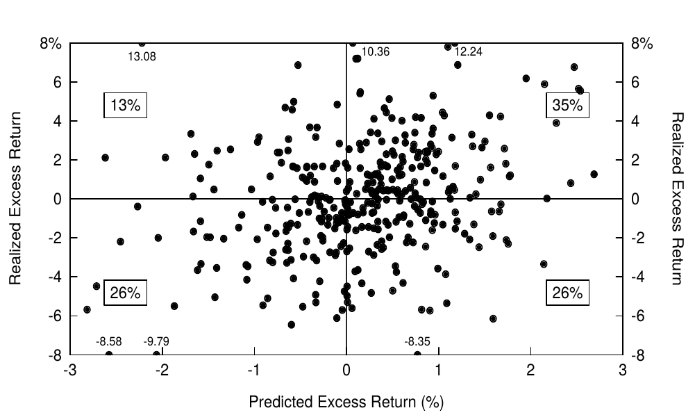
Figure 4.5 Realized Excess Return versus Predicted Excess Return, 1965-95

The relation between the predicted and the realized excess returns in Figure 5 may not appear very impressive, reflecting the fact that most of the short-term fluctuations in excess bond returns are unpredictable. Perhaps the long-term fluctuations are more predictable; averaging many monthly returns will smooth the return series and may increase the share of the predictable returns. Our unpublished analysis shows that in a scatter plot of the subsequent 12-month realized excess bond returns on the predicted excess returns, 84% of the observations are in the upper-right quadrant or in the lower-left quadrant. Moreover, the correlation between the out-of-sample predictions and the subsequent 12-month excess returns is 0.57, much larger than the 0.26 correlation between these predictions and the subsequent monthly excess returns.

图5中预测和实现的超额回报之间的关系可能不是非常令人印象深刻，这反映了大多数债券超额回报的短期波动是不可预测的事实。也许长期波动更可预测； 将许多月度回报平均会平滑回报序列，并可能增加回报的可预测性。我们未发表的分析显示，后续12个月的实现债券超额回报关于预测超额回报的散点图中，84%的观察值在右上象限或左下象限。此外，样本外预测与好后续12个月超额回报之间的相关性为0.57，远大于这些预测与后续月度超额回报之间0.26的相关性。

Figure 6 displays a time series plot of the monthly predicted excess returns and the subsequent 12-month average excess returns. We also plot the time series of each predictor variable in Figure 7, to better identify the sources of fluctuations in expected excess bond returns. Figure 6 shows that the predictions track the movements in the realized bond returns reasonably well. Both series in Figure 6 were low in the 1960s and 1970s and exceptionally high in the 1982-85 period, reflecting slow-moving changes in the real yield and in the term spread. Aside from these broad movements, both series exhibit apparent business cycle patterns: The predicted returns tend to increase during cyclical contractions such as those in 1970, 1974 and 1982. Figure 7 shows that these increases in expected returns as well as those in the aftermath of the 1987 stock market crash (when a recession was widely expected) and in the most recent recession (1990 Gulf War) coincide with inverse wealth spikes, that is, with poor stock market performance. These patterns are consistent with our hypothesis that wealth-dependent risk aversion causes the required bond risk premium to vary over time with economic conditions. However, the negative excess return forecasts in the 1960s, 1973-74, 1979-80, and 1989 are difficult to interpret; most bond market participants think that the bond risk premium is always positive. Finally, it is worth noting that the forecasting model is currently quite bearish. The excess bond return predictions have been negative since the end of May 1995, mainly because of the strong stock market (low inverse wealth) and the relatively flat yield curve (low term spread).^[8]

图6显示了月度预测超额回报和后续12个月平均超额回报的时间序列图。我们还在图7中绘制每个预测变量的时间序列，以更好地确定预期债券超额回报波动的来源。图6显示，预测相当好地跟踪实现债券回报的变动趋势。图6中的两个系列在1960年和1970年代都很低，在1982-85年期间异常高，这反映了实际收益率和期限利差的缓慢变化。除了这些大的趋势变化之外，两个系列都展示了明显的商业循环模式：预测的回报在周期性经济收缩（如1970年，1974年和1982年）期间趋于上涨。图7显示，预期回报的增长发生在1987年股市崩盘（当经济衰退得到广泛预期）和最近的衰退（1990年海湾战争）之后，与逆财富的增长（即股市表现不佳）相反。这些模式与我们的假设一致，即财富依赖风险厌恶导致要求的债券风险溢价随着不同时期的经济状况而变化。然而，1960年代，1973-74年，1979-80年和1989年的负超额回报预测难以解释；大多数债券市场参与者认为，债券风险溢价总是正的。最后，值得注意的是，预测模型目前看跌。自1995年5月底以来，债券超额回报预测为负，主要是由于股市强劲（低逆财富）和收益率曲线相对平坦（低期限利差）。

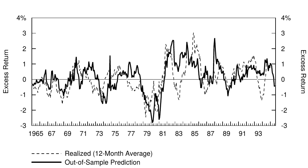
Figure 4.6 Predicted Excess Bond Return and Subsequent Realized 12-Month Excess Bond Return, 1965-95

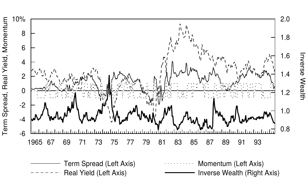
Figure 4.7 Historical Levels of the Predictor Variables, 1965-95

INVESTMENT IMPLICATIONS OF BOND RETURN PREDICTABILITY

债券回报预测的投资应用

Exploiting Return Predictability by Using Dynamic Investment Strategies

利用动态投资策略挖掘回报的可预测性

Even if the predictor variables appear to have some ability to forecast excess bond returns in an out-of-sample setting, should investors care about these findings? For portfolio managers, the key question is whether investment strategies that exploit the return predictability produce economically significant profits. In this section, we first describe the implementation of such dynamic investment strategies and then present extensive analysis of their historical performance. In particular, we compare their historical returns to the returns of static strategies that have a constant portfolio composition regardless of economic conditions. One goal is to show that the information in the yield curve and in other predictors could have been used to enhance long-run returns. Another goal is to provide a tool kit to evaluate the future profitability of any forecasting strategy and a set of critical questions (economic reason for success, stability of success, sensitivity to transaction costs and to risk adjustment) that an investor should ask when faced with backtest evidence of an apparently attractive investment strategy.

即使预测变量似乎有一定的能力来预测样本外的债券超额回报，投资者是否应该关心这些研究结果？对于投资组合经理来说，关键问题是利用回报可预测性的投资策略是否会带来经济上的显着利润。在本节中，我们首先描述这种动态投资策略的实现，然后对其历史表现进行广泛分析。特别地，我们比较他们的历史回报与静态策略（无论经济状况如何，该策略具有不变的投资组合）的回报。一个目标是显示收益率曲线和其他预测指标中的信息可能被用来增加长期回报。另一个目标是提供一个工具包，以评估任何预测性策略的未来盈利能力；以及回测显示一个投资策略非常有吸引力时，投资者应询问的一系列关键问题（策略成功的经济原因、策略成功的稳定性、交易成本的敏感性和风险调整）。

The static strategies are called "always-bond" and "bond-cash combination." The former strategy involves always holding a 20-year Treasury bond, while the latter involves always holding 50% of the portfolio in cash (one-month Treasury bill) and 50% in the 20-year Treasury bond, with monthly rebalancing. The dynamic strategies adjust the allocation of the portfolio between cash and the 20-year Treasury bond each month, based on the predicted value of next month's excess bond return. The two dynamic strategies are called "scaled" and "1/0." The 1/0 strategy is simpler: It involves holding one unit of the 20-year bond when its predicted excess return is positive and zero when it is negative (thus, holding cash). This approach ignores information about the magnitude of the predicted excess return. In contrast, the scaled strategy involves buying more long-term bonds the larger the predicted excess return is. Specifically, investors should buy or short-sell the long-term bond in proportion to the size of the predicted excess return.^[9]

静态策略分别被称为“纯债券策略”和“债券-现金组合策略”。前一项策略总是持有20年期国债，而后者则总是持有50%的现金（一月期国库券）和50%的20年期国债，每月重新平衡一次。动态策略根据下个月债券超额回报的预测值，每月调整现金与20年期国债之间的投资组合分配。两种动态策略称为“比例策略”和“1/0策略”。1/0策略比较简单：当预测的超额回报为正值时，持有20年期债券的比例为1，否则为零（此时持有现金）。这种方法忽略了有关预测超额回报的幅度的信息。相比之下，预期超额回报幅度越大，比例策略将持有越多的长期债券。具体来说，投资者应该根据预期的超额回报的大小按比例购买或卖空长期债券。

Strategy returns are expressed in excess of the one-month bill return. For investors who have investable funds, each strategy's total return would be approximately equal to its excess return plus the one-month bill's return (which is the same number for all of the strategies). For arbitrage traders who only hold self-financed positions, the reported excess return can be interpreted as the total return of their "zero-net-investment" position —— to the extent that they can finance their positions using the one-month bill rate.

策略回报中减去了一月期国库券的收益率。对于拥有可投资资金的投资者，每个策略的总回报将近似等于其超额回报加上一月期国库券收益率（对所有策略相同）。对于只有自融资头寸的套利交易者，报告的超额回报可以解释为“零净投资”头寸的总回报——只要他们能够以一月期国库券收益率为自己的头寸融资。

Figure 8 shows, for each strategy, the annualized average excess return, the volatility of excess returns as well as the Sharpe ratio. Note that a cash portfolio earns zero excess return by definition; it is equivalent to holding cash financed with cash. Therefore, the 50-50 bond-cash combination has exactly half of the excess return and volatility of the always-bond strategy. The static strategies yielded only insignificant excess returns over the sample period. In other words, long-term bonds and short-term bonds earned quite similar average returns. The dynamic strategies performed much better. The scaled strategy earned almost a 9% average annual excess return while the 1/0 strategy earned about half of that. Also the rewards to volatility (Sharpe ratios) of the dynamic strategies are much larger than those of the static strategies.^[10]

图8显示了每个策略的年化平均超额回报，超额回报的波动率以及夏普比率。请注意，现金组合根据定义获得零超额回报；相当于持有现金资金。因此，50比50的债券-现金组合的超额回报和波动率只是纯债券策略的一半。在样本期，静态策略只能产生微不足道的超额回报。换句话说，长期债券和短期债券的平均回报大致一样。动态策略表现更好，比例策略的平均年化超额回报达到9%，而1/0策略大约获得其一半的回报。动态策略波动率的回报（夏普比率）也远远大于静态策略。

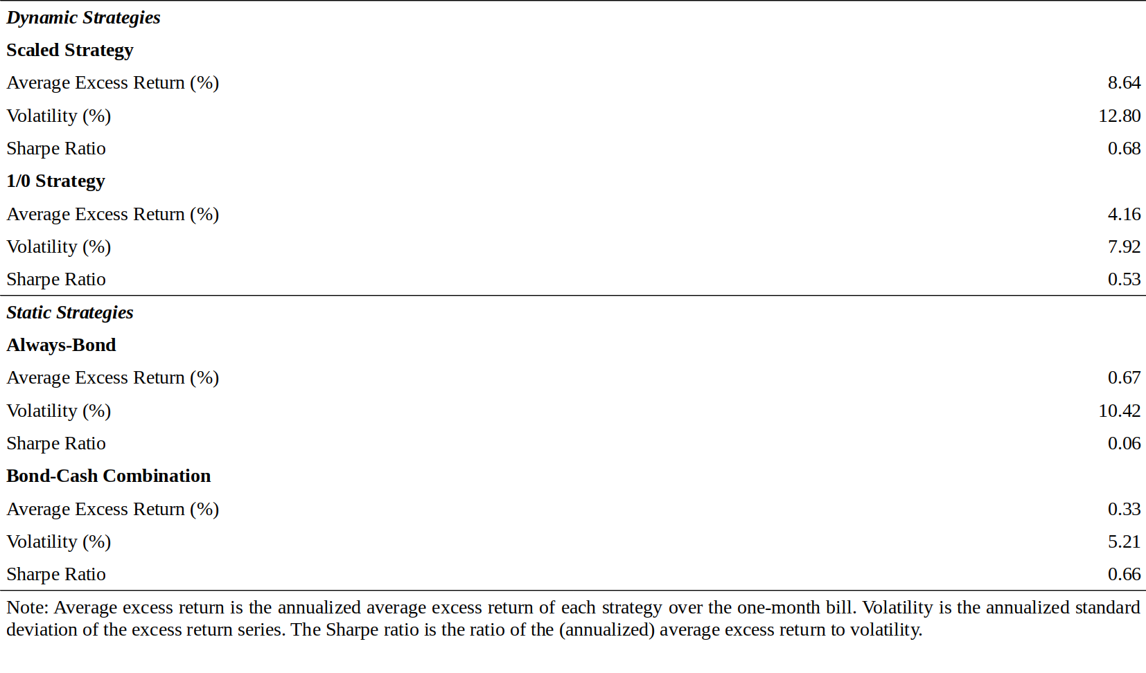
Figure 4.8 Performance of Self-Financed Dynamic and Static Investment Strategies, 1965-95

We can compare the performance of the dynamic strategies in Figure 8 with the performance of a dynamic strategy that uses only the information in the term spread. The scaled strategy would have earned 3.87% per annum and the 1/0 strategy 2.96% per annum if the out-of-sample forecasts had been based on the term spread alone. Comparison with the average returns in Figure 8 (8.64% and 4.16%) indicates that the marginal value of the other predictors has been substantial. It is also worth noting that the scaled strategy would have earned 11.15% per annum and the 1/0 strategy 4.94% per annum if the predictions had been based on the in-sample estimates from the regression of excess bond returns on the four predictors. The difference between the performance of the in-sample and the out-of-sample forecasts may reflect the data-snooping bias.

我们可以比较图8中动态策略与仅使用期限利差中信息的动态策略的表现。如果样本外预测仅基于期限利差，则比例策略的回报是3.87%，而1/0策略的回报是2.96%。与图8的平均回报（8.64%和4.16%）的比较表明，其他预测因子的边际价值已经很大。还有一点值得注意的是，如果预测基于四个预测因子（来自债券超额回报回归分析的样本内估计值），那么比例策略的年化回报是11.15%，1/0策略的年化回报是4.94%。样本内和样本外预测的表现差异可能会反映了数据窥探偏差。

Stability of the Predictive Relations

预测的稳定性

The analysis above shows, first, that over the past 30 years, our predictors have been able to forecast near-term bond returns and, second, that strategies that exploit such predictability have earned economically meaningful profits. In this section, we examine the stability of these findings over time, if the predictive ability and exceptional performance arise from a couple of extreme observations, we become skeptical about the reliability of these findings. However, if the observed relations are consistent across subperiods, we think that they are less likely to be spurious. Thus, we become more comfortable in expecting that the historical experience (good predictive ability and the dynamic strategies exceptional performance) will be repeated in the future. We will study three types of evidence: Rolling correlations; subperiod analysis of average returns; and cumulative performance of various investment strategies.

上述分析显示，首先，在过去30年中，我们的预测指标已经能够预测近期债券回报；其次，利用这种可预测性的策略获得了经济上有意义的利润。在本节中，我们将考察这些发现随时间的稳定性，如果预测能力和出色表现来自若干极端观察结果，我们将对这些发现的可靠性持怀疑态度。然而，如果所观察到的关系在不同子时段是一致的，我们认为它们不太可能是虚假的。因此，我们希望将来会再次重复历史经验（良好的预测能力和动态策略出色表现）。我们将研究三种证据：滚动相关性、子时段平均回报分析和各种投资策略的累积表现。

Figure 9 shows that estimated rolling 60-month correlations between the predictors and the subsequent bond return are not constant, but they are positive in most subperiods. In the 1990s, the real yield and momentum have had little forecasting ability, but both the term spread and inverse wealth have had predictive correlations near 20%. The combined predictor tends to have better forecasting ability than any of the individual predictors. Similar subperiod analysis shows that the frequency of correctly predicting the sign (+/-) of the next month's excess bond return is reasonably stable and near 60%.

图9显示，预测值与随后的债券回报之间的60个月滚动相关性不是恒定的，但在大多数子时段中它们是正的。1990年代，实际收益率和动量几乎没有预测能力，但是期限利差和逆财富有近20%的预测相关性。组合预测往往具有比任何单个预测因子更好的预测能力。类似的子时段分析显示，正确预测下个月债券超额回报的符号（+/-）的频率相当稳定，接近60%。

Figure 4.9 Rolling 60-Month Correlation of Various Predictors with Subsequent Excess Bond Return, 1965-95

Figure 10 reports the statistics from Figure 8 for three decade-long subsamples and for the 1990s subperiod. It is encouraging to see that the observed patterns are stable across decade-long subsamples. In particular, both dynamic strategies outperform the bond-cash combination strategy by at least 200 basis points in all subperiods.

图10报告了图8中三个十年长的子样本和1990年代以来的统计。令人鼓舞的是，观察到的模式在十年之久的子样本中是稳定的。特别是，两种动态策略在所有子时段中优于债券-现金组合策略至少200个基点。

Figure 4.10 Subperiod Performance of Various Investment Strategies, 1965-95

The most informative way to display the stability of a predictive relation is to plot the cumulative wealth of an investment strategy that exploits the predictive relation. Such a graph shows how the profits from the strategy grow over time. Note that the cumulative wealth of an ideal perfect-foresight strategy would never decline; moreover, it should also be rising faster than the cumulative wealth of any competing strategies. Alternatively, we can plot the relative performance of two investment strategies, and again, the line representing a perfect-foresight strategy should always be rising (or flat if it matches the performance of the other strategies).

显示预测关系稳定性最有效的方法是绘制利用预测关系的投资策略的累积财富。这样的图表显示了策略的利润如何随着时间的推移而增长。请注意，理想的完美预测策略的累积财富永远不会下降；此外，它也应该比任何竞争策略的累积财富增长快得多。或者，我们可以绘制两种投资策略的相对表现，代表完美预测的策略的累积财富曲线应该总是在上升（或平坦，如果与其他策略的表现相一致）。

Figure 11 shows the cumulative wealth growth of both dynamic strategies and the always-bond strategy (plotted on a log-scale where constant percentage growth produces a straight line). Because the lines cumulate each strategy's monthly returns in excess of cash (the one-month bill), we also can interpret these lines as relative performance versus cash. Figure 12 measures the relative performance of the two dynamic strategies versus a more realistic benchmark, a 50-50 combination of cash and the long-term bond. These graphs show that the dynamic strategies have had a consistent ability to outperform the static strategies. The scaled strategy earned very high returns in the late 1970s and early 1980s by short-selling the long-term bond during the bear market. During the subsequent bull market, the dynamic strategies have earned similar returns as the static bondholding strategy. This result must be viewed as satisfactory, because this bull market has been exceptionally strong and long, making long-term bond returns a difficult target to beat. Figures 11 and 12 show that the dynamic strategies never underperformed the benchmark static strategies for an extended period. And what about the recent experience? The dynamic strategies have outperformed the static strategies in the 1990-95 period —— see Figure 10 —— but last year (1994) both dynamic strategies underperformed the cash-bond combination because they remained in long-term bonds throughout a period of rising rates.

图11显示了动态策略和纯债券策略的累积财富增长（绘制在对数标度上，其中恒定百分比增长产生一条直线）。由于这些曲线将每个策略月回报超过现金（一月期国库券）的部分累积，我们也可以将这些线作为与现金的相对表现。图12表现了两种动态策略的相对表现，关于更现实的基准——50比50的现金-长期债券的组合。这些图表显示，动态策略具有一致超越静态策略的能力。1970年代末和80年代初期，通过在熊市中卖出长期债券，比例策略获得了很高的回报。在随后的牛市中，动态策略获得了与静态债券持有策略相似的回报。这个结果必须被认为是令人满意的，因为这个牛市已经非常强劲和长久，使得长期债券回到了难以实现的高度。图11和图12显示，长期以来，动态策略从未逊于基准静态策略。最近的经验呢？动态策略优于1990-95年期间的静态策略（见图10），但去年（1994年）动态策略相对于现金-债券组合的表现不佳，因为在加息期间持有了长期债券。

Figure 4.11 Cumulative Wealth Growth from Three Self-Financed Strategies, 1965-95

Figure 4.12 Dynamic Strategies' Relative Performance versus Bond-Cash Combination, 1965-95

Other Critical Considerations

其他关键注意事项

The backtest results suggest that bond investors could enhance their performance substantially by exploiting the forecasting ability of the term spread, the real yield, inverse wealth, and momentum. However, historical success does not guarantee future success. We stress that any reported findings of apparently profitable investment strategies should be subjected to a set of critical questions. We already addressed the important concern about data-snooping bias —— we used out-of-sample forecasts, we restricted the predictors to economically well-motivated variables, and we ensured that the observed findings are relatively stable across subperiods. Other reservations include the sensitivity of the findings to transaction costs and to risk adjustment.

回测结果表明，债券投资者可以通过利用期限利差、实际收益率、逆财富和动量的预测能力大幅度提高其业绩。然而，历史成功并不能保证未来的成功。我们强调，任何报告中明显盈利的投资策略的结果应该考虑到一系列关键问题的影响。我们已经解决了对数据窥探偏差的关切——通过使用了样本外预测，将预测因子限制在经济含义良好的变量中，我们确保观察到的发现在不同时期相对稳定。其他剩余问题包括研究结果对交易成本的敏感性和风险调整。

Transaction costs will reduce the profitability of any investment strategy. However, government bonds have such small transaction costs for institutional investors that their impact on the reported returns should be small. In particular, the results of the 1/0 strategy are hardly affected because this strategy involves very infrequent trading —— on average 1.5 trades per year. The scaled strategy is more transaction intensive, and it also involves short-selling. Thus, the reported results are somewhat exaggerated.

交易成本将降低任何投资策略的盈利能力。然而，对机构投资者来讲国债的交易成本较低，对报告中的回报影响较小。特别是，1/0策略的结果几乎不受影响，因为这个策略涉及非常少的交易——平均每年1.5笔交易。比例策略交易密集，也涉及到卖空。因此，报告的结果有些夸张。

The dynamic strategies offer higher returns than the static strategies, but they excel even more when the comparison is made between risk-adjusted returns. First, if risk is measured by the volatility of returns, the Sharpe ratios in Figure 8 provide a risk-adjusted comparison. The volatility of the scaled strategy is higher than that of the static bond strategy, but its reward-to-volatility ratio is more than ten times higher. The volatility of the 1/0 strategy is lower and the average return higher than that of the static always-bond strategy. Second, if investors are concerned with downside risk, the dynamic strategies will look even better. The historical success of these strategies partly reflects their ability to avoid long-term bonds during bear markets. For example, we can infer from Figure 5 that the 1/0 strategy underperformed cash in only 26% of the months in the sample (outperforming it 35% of the time and matching its performance 39% of the time when the predicted excess return was negative and the strategy involved holding cash). However, if the return predictability reflects a time-varying risk premium, it is possible that the abnormally high returns of the dynamic strategies reflect only a fair compensation for taking tip additional risk at times when either the amount of risk or risk aversion is abnormally high.

动态策略提供比静态策略更高的回报，但是当对风险调整后的回报进行比较时，这些策略更加突出。首先，如果风险是通过回报的波动率来衡量的，图8中的夏普比率提供了风险调整后的比较。比例策略的波动回报高于静态债券策略，但其回报-波动率比要高出十倍以上。同静态纯债券策略相比，1/0战略的波动率更低和平均回报更高。第二，如果投资者担心下行风险，动态策略表现会更好。这些策略的历史性成功部分反映了在熊市期间避免持有长期债券的能力。例如，我们可以从图5推断，1/0的策略在样本中只有26%的月份落后于现金（策略优于现金的时间超过了35%，39%的时间与现金一致，如果预期超额回报为负，这时策略为持有现金）。然而，如果回报可预测性反映了时变的风险溢价，则动态策略的异常高回报可能仅反映在风险或风险厌恶程度异常高的时候对额外风险的公允补偿。

In spite of the apparent attractiveness of the dynamic strategies, few investors have tried to systematically exploit the predictability of bond returns. For those investors who venture to do that, this fact is good news. The profit opportunities are not likely to be "arbitraged away” any time soon. One major reason is that these strategies are not riskless arbitrages —— they involve a lot of short-term risk because the forecasts are wrong 40% of the time. Nonetheless, 60-40 odds are attractive in competitive financial markets. Therefore, what could make investors forego the exceptionally favorable odds that the dynamic strategies offer? Here are some possible explanations.

尽管动态策略具有明显的吸引力，但很少有投资者试图系统地利用债券回报的可预测性。对于那些冒险这样做的投资者来说，这个事实是个好消息。利润机会不会很快被“吃光”。其中一个主要原因是这些策略不是无风险的套利——它们涉及很多短期风险，因为40%的预测是错误的。尽管如此，在竞争激烈的金融市场有60比40的胜算依旧是有吸引力的。但是投资者为什么仍然放弃动态策略提供的非常有利的可能性呢？这里有一些可能的解释：

• Many investors prefer the more subjective interest rate forecasting approach even if its track record is rarely good. Other investors believe that market fluctuations cannot be predicted; thus, they do not want to take any market directional positions. Such investors would attribute our predictability findings to data snooping or to events that the market was expecting but that were not realized during the sample period.

• 许多投资者喜欢采用更主观的收益率预测方法，即使其历史记录不佳。其他投资者认为市场波动无法预测；因此，他们不想持有任何市场指向性的仓位。这样的投资者将我们的可预测性研究结果归因于数据窥探或市场预期但在抽样期间尚未实现的事件。

• The potential losses from such strategies may loom larger than the potential gains. The short-term risk in the dynamic strategies may expose portfolio managers to substantial career risk^[11] even if the strategies are likely to outperform in the long run. Moreover, the losses may have a tendency to occur at especially unpleasant times.^[12] The dynamic strategies high expected return may be a reward for such discomforts.

• 这些策略的潜在损失可能大于潜在回报。动态策略中的短期风险可能使投资组合经理面临重大的职业风险，即使这些策略长期可能跑赢市场。此外，损失可能会在特别令人不快的时候发生。动态策略的高预期回报可能是对这种不快的回报。

Even if some investors find the strategy too mechanical or too risky to be used systematically, they may want to use it selectively. For example, they may want to use the strategy only when the signal is very strong. What do historical data say about such an approach? The fact that the scaled strategy outperforms the 1/0 strategy suggests that the magnitude of the predicted excess return contains valuable information beyond the sign. Figure 13 studies whether the return predictions become more reliable when the forecast deviates much from zero. It also reports the average returns at different levels of predicted excess returns. We can see that the frequency of correct sign forecasts is only weakly related to the absolute value of the forecast. The average excess returns show clearer patterns: large negative values when the predictions are very negative and large positive values when the predictions are very positive.

即使一些投资者发现这个策略太机械化风险太大，不能系统地使用，他们可能希望有选择地使用它。例如，他们可能只想在信号非常强的时候使用策略。历史数据对这种做法有什么看法？比例策略优于1/0策略的事实表明，预测超额回报的幅度包含的信息比单纯预测符号有价值。图13研究了当预测显著不为零时，回报预测是否变得更可靠。它还报告了不同预测超额回报水平的平均回报。我们可以看到，正确预测符号的频率与预测绝对值仅有很弱的相关性。平均超额回报显示了更清晰的模式：当预测非常大的时候，预测结果也非常大，反之亦然。

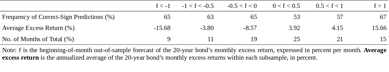
Figure 4.13 Impact of the Forecast Signal’s Strength on the Return Predictability, 1965-95

Impact of Investment Horizon

投资期限的影响

We suggested above that the dynamic strategies may involve an unacceptably high risk of short-term underperformance (see footnote 11). However, the long-run performance of these strategies should make them very appealing for investors who can afford to take a long investment horizon. In this section, we focus on the impact of investment horizon on the attractiveness of the dynamic strategies. The crucial question we address is: How long a horizon is long enough for investors to be confident that these strategies outperform cash and / or bonds? Recall that the out-of-sample forecasts of next month's excess bond return have a correct sign in 61% of the months in the sample (see Figure 5). Increasing the investment horizon from one month makes the dynamic strategies look better and better. For example, Figure 14 shows that the scaled strategy outperformed the always bond strategy in 23 calendar years out of 30 in this sample, and the 1/0 strategy underperformed the always bond strategy in only two calendar years (and matched it in ten other years when it kept holding the long-term bond).

我们上面提出，动态策略可能会带来短期表现不佳的风险（见脚注11）。然而，这些策略的长期表现应该使他们对能够承受长期投资的投资者非常具有吸引力。在本节中，我们重点关注投资期限对动态策略吸引力的影响。我们提出的关键问题是：投资期限要多长时间，投资者才能确定这些策略优于持有现金或债券？回想一下，61%的月份中债券超额回报的样本外预测是正确的（见图5）。增加投资期限使动态战略看起来越来越好。例如，图14显示，在这个样本中，比例策略在30年中的23年中超过了纯债券策略，而1/0策略仅在两年中表现不如纯债券战略（其中10年表现一致，因为1/0策略一直持有长期债券）。

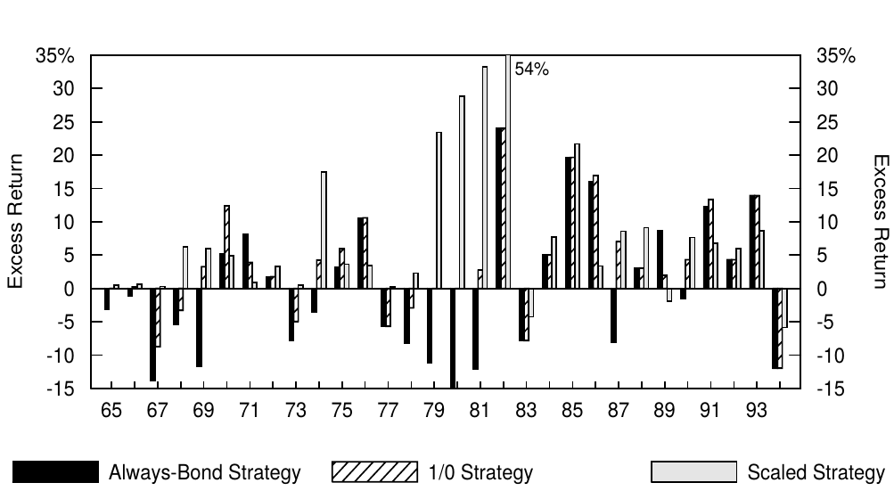
Figure 4.14 Annual Excess Returns of Three Self-Financed Strategies, 1965-94

Figure 15 shows —— for various horizons —— the frequency at which the dynamic strategies outperformed or matched cash, the long-term bond or both. The longer horizon numbers are based on overlapping monthly data.^[13]

图15显示了不同期限动态策略跑赢或持平现金、长期债券或两者兼而有之的频率。更长的期限数字是基于重叠的月度数据。

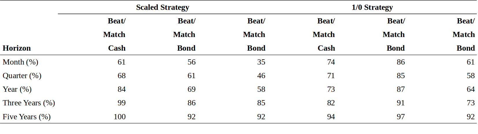
Figure 4.15 Impact of the Horizon Length to the Strategy’s Success Rate, 1965-95

Focusing on the toughest comparison, the dynamic strategies outperformed both bonds and cash in roughly 60% of the one-year periods in the sample. For the three-year horizon, the frequency increases to about 80% of the sample, and for the five-year horizon to 92%. In a way, the dynamic strategies would have provided a free outperformance option for long-term investors. Figure 16 illustrates this point by showing the rolling 36-month excess return for each strategy. If the dynamic strategies outperform both cash and bonds, their excess returns should lie above the excess returns of cash (zero line) and the always-bond strategy. This is roughly what we see in the graph. We conclude that although historical analysis provides no guarantee about the future and although backtest results are rarely achieved in real-world investments, the odds in favor of the dynamic strategies appear excellent for three- to five-year investment horizons.

注意其中最艰难的比较，在一年期间动态策略在样本中大约60%的时间内表现优于债券和现金。在三年期的时间里，比例上升到大约80%，五年期为92%。在某种程度上，动态策略将为长期投资者提供一个免费出色表现的选项。图16显示了每个策略的36个月滚动超额回报。如果动态策略优于现金和债券，其超额回报应超过现金超额回报（零值线）和纯债券策略。这大概是我们在图表中看到的。我们得出下面的结论，虽然历史分析不能保证未来，并且在现实世界投资中很少实现回测结果，但动态策略的表现在三到五年的投资期限中依然显得非常出色。

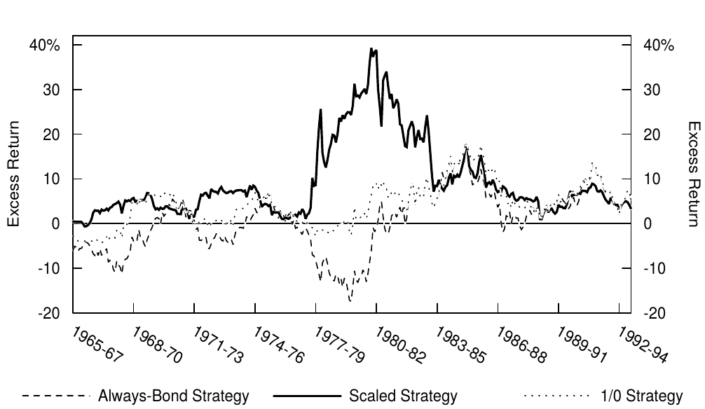
Figure 4.16 Rolling 36-Month Excess Returns of Three Self-Financed Strategies, 1968-95

CONCLUDING REMARKS

结论

In this report, we have shown that long-term bond returns are predictable. A set of four predictors —— yield curve steepness, real bond yield, recent stock market performance, and bond market momentum —— is able to forecast 10% of the monthly variation in long-term bonds' excess returns. Thus, when making inferences about the yield curve behavior, bond market analysts should not assume that the bond risk premium is constant over time. The bond risk premium may be small, on average, but we can identify in advance periods when it is abnormally large or small. A forecasting model gives us an estimate of the near-term bond risk premium —— but even the best models' estimates are subject to various errors. Nevertheless, such models can be valuable tools for long-term investors. We find that dynamic investment strategies that exploit the bond return predictability have consistently outperformed static investment strategies over long investment horizons.

在本报告中，我们已经表明长期债券回报是可以预测的。四个预测因子——收益率曲线陡峭程度、实际债券收益率、近期股市表现以及债券市场动量，能够预测长期债券超额回报月度变动的10%。因此，当对收益率曲线行为作出推论时，债券市场分析师不应假定债券风险溢价随时间不变。债券风险溢价平均可能很小，但我们可以提前确定异常大或小的期间。预测模型给出了近期债券风险溢价的估计，但即使是最佳模型的估计也有各种错误。然而，这种模型可以成为长期投资者的有力工具。我们发现，在长投资期限中利用债券回报可预测性的动态投资策略一直优于静态投资策略。

There are many ways to implement investment strategies that exploit return predictability. This report presents two dynamic strategies (scaled and 1/0) that shift funds between cash and a long-term bond based on the sign and the magnitude of the return prediction. One alternative way to implement the strategy is through active duration management using on-the-run Treasury bonds or bond futures. An investor could modify his portfolio duration dynamically based on the magnitude of the return prediction. The range of durations would depend on the investor's risk aversion level and on his confidence in the proposed strategy. Figure 17 gives an example of how various investor types (aggressive, moderate, conservative) with a neutral benchmark duration of four years could vary their portfolios target duration with economic conditions. Of course, more conservative implementation would reduce the potential for return enhancement.

有许多方法来实施利用回报可预测性的投资策略。本报告提出了分别基于回报预测的符号和幅度的两种动态策略（比例策略和1/0策略），两种策略通过现金和长期债券之间的切换来实现。实施策略的另一种方法是通过使用活跃国债或债券期货进行积极的久期管理。投资者可以根据回报预测的幅度动态修改投资组合的久期。久期的大小将取决于投资者的风险厌恶水平以及对策略的信心。图17给出了一个例子，说明了以四年为中性基准久期的基础上，各种类型的投资者（激进型、中间型和保守型）如何根据其经济条件改变投资组合的目标久期。当然，更保守的措施将会降低回报增加的潜力。

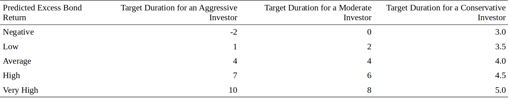
Figure 4.17 Implementing the Strategy: From Return Predictions to Target Portfolio Durations

The analysis in this report focuses on the predictability of the excess return of a 20-year US Treasury bond using four predictor variables. Obviously, the analysis could be extended in various directions:

本报告的分析重点是四个预测变量关于20年期美国国债超额回报的可预测性。显然，分析可以在各个方向扩展：

• One might improve the forecasts by using a broader set of predictors or by combining their information in a more sophisticated way than a simple linear regression. However, our small set of predictors may have more robust forecasting ability in an out-of-sample setting than a broad predictor set would. We have not found other predictors that consistently and significantly improve the forecasting ability of our four-predictor model.

• 人们可以通过使用更广泛的预测因子来改进预测，或者通过以比简单的线性回归更复杂的方式组合它们的信息来改善预测。然而，我们的少量预测因子可能比大量的预测因子在样本外有更稳健的预测能力。我们还没有发现其他预测因子可以一致显着地提高四因子预测模型的预测能力。

• One can examine the return predictability over a shorter investment horizon than one month. The predictors we use above may be too slow-moving for short-term traders. They often prefer to trade either on their fundamental views or on momentum and overreaction effects (price trends and reversals) or on other technical factors (supply effects and portfolio flows). It might be a good idea to subject even these trading approaches to the performance evaluation proposed in this report.

• 人们可以在比一个月更短的投资期限内检查回报的可预测性。我们上面使用的预测因素对于短期交易者来说可能太慢了。他们往往倾向于根据其基本面观点或动量和过度反应（价格走势和逆转）或其他技术因素（供应效应和投资组合流动）进行交易。将这些交易方法应用于本报告中提出的表现评估可能是个好主意。

• One can examine the return predictability of other government bonds. We show elsewhere that our predictors can also forecast the excess returns of shorter-maturity bills and bonds in the United States and that similar variables forecast international bond returns (see the Literature Guide).

• 可以检查其他政府债券的回报可预测性。我们在其他地方展示，我们的预测指标也可以预测美国短期国库券和债券的超额回报，类似的变量也可以预测国际债券回报（见文献指南）。

• One can examine the predictability of the relative performance of various bond market sectors and markets (changes in the yield spreads across maturities, across market sectors and across countries). In this report, we combine the information in the term spread and other predictors to improve our forecasts of excess bond returns. In a similar way, we could combine the information in mean-reverting yield spreads and in other predictors to develop better relative value indicators. The tools presented in this report also can be used to evaluate the forecasting performance of various relative value indicators.

• 可以检查各种债券市场部门和市场的相对表现的可预测性（不同期限、市场和国家的收益率差异的变化）。在本报告中，我们将期限利差和其他预测因子的信息相结合，以改善我们对债券超额回报的预测。以类似的方式，我们可以将均值回归利差中的信息与其他预测因子结合起来，以开发更好的相对价值指标。本报告提供的工具也可用于评估各种相关价值指标的预测效果。

LITERATURE GUIDE

文献指南

Extensive literature exists discussing the predictability of bond, stock, and currency returns and the dynamic (or "tactical asset allocation") strategies that try to exploit the return predictability. We focus here on studies about bond return predictability.

众多文献讨论了债券、股票和货币回报的可预测性，以及试图利用回报可预测性的动态(或“战术资产配置”)策略。在这里，我们着重关注的是关于债券回报可预测性的研究。

On the Predictability of US Bond Returns and on the Concept of Time-Varying Risk Premium

关于美国市场上债券的回报可预测性以及时变的风险溢价

• Keim and Stambaugh, "Predicting Returns in the Bond and Stock Markets," Journal of Financial Economics, 1986.
• Fama and Bliss, "The Information in Long-Maturity Forward Rates," American Economic Review, 1987.
• Fama and French, "Business Conditions and Expected Returns on Stocks and Bonds," Journal of Financial Economics, 1989.
• Jones, "Can a Simplified Approach to Bond Portfolio Management Increase Return and Reduce Risk?", Journal of Portfolio Management, 1992.
• Campbell and Ammer, "What Moves Stock and Bond Markets?," Journal of Finance, 1993.
• Campbell, "Some Lessons from the Yield Curve," National Bureau of Economic Research working paper #5031, 1995.
• Tyson, "Estimation of the Term Premium," Fixed-Income Investment: Recent Research, ed. Ho, 1995.

On the Predictability of International Bond Returns

关于国际市场上债券的回报可预测性

• Mankiw, "The Term Structure of Interest Rates Revisited," Brookings Papers on Economic Activity, 1986.
• Bisignano, "A Study of Efficiency and Volatility in Government Securities Markets," Bank for International Settlements, 1987.
• Ilmanen, "Time-Varying Expected Returns in International Bond Markets," Doctoral dissertation, Graduate School of Business, University of Chicago, 1994.
• Ilmanen, "Time-Varying Expected Returns in International Bond Markets," Journal of Finance, 1995.
• Ilmanen, "When Do Bond Markets Reward Investors for Interest Rate Risk?," Journal of Portfolio Management (forthcoming), 1996.

On Wealth-Induced Variation in the General Risk Aversion Level and on Other Explanations for the Return Predictability

关于一般风险规避水平上的财富引发的变化以及其他关于回报可预测性的解释

• Marcus, "An Equilibrium Theory of Excess Volatility and Mean Reversion in Stock Market Prices," National Bureau of Economic Research working paper #3106, 1989.
• Froot, "New Hope for the Expectations Hypothesis of the Term Structure of Interest Rates," Journal of Finance, 1989.
• Sharpe, "Investor Wealth Measures and Expected Return," in the seminar proceedings from Quantifying the Market Risk Premium Phenomenon for Investment Decision Making, The Institute of Chartered Financial Analysts, 1990.
• Chen, "Financial Market Opportunities and the Macroeconomy," Journal of Finance, 1991.
• DeBondt and Bange, "Inflation Forecast Errors and Time Variation in the Term Premia," Journal of Financial and Quantitative Analysis, 1992.

---

1. We define the bond risk premium as the near-term (say, one-month) expected return of a long-term government bond in excess of the return of the near-term riskless asset (say, the one-month Treasury bill). The long-run bond risk premium is the long-run average expected return of a long-duration strategy in excess of the long-run average expected return of a short-duration strategy. It may differ from the (near-term) bond risk premium if the latter is abnormally high or low. Our definition of bond risk premium encompasses any expected return differential between a long-term bond and the near-term riskless bond, whether it is actually related to risk or to some technical factor. For this reason, we often call the bond risk premium, more neutrally, the "expected excess bond return."
   我们将债券风险溢价定义为长期政府债券的近期（比如一个月）预期回报超过近期无风险资产回报（例如一月期国库券）的部分。长期债券风险溢价是长久期策略的长期平均预期回报超过短久期策略的长期平均预期回报的部分。如果后者异常高或低，则可能与（近期）债券风险溢价有所不同。我们对债券风险溢价的定义包括长期债券与短期无风险债券之间的任何预期回报差，无论其实际上与风险或某些技术性因素相关。因此，我们经常称债券风险溢价为“预期债券超额回报”。 ↩︎

2. Moving average trading rules are perhaps the most popular trend-following strategies among traders. Such strategies are profitable if the market moves more in trends than sideways within a trading range. Even though academic research in the 1960s and 1970s found that common technical trading rules do not consistently outperform buy-and-hold strategies, more recent studies have shown that some trend-following strategies are profitable, especially in the foreign exchange market. See, for example, "Technical Trading: When It Works and When It Doesn't," William Silber, Journal of Derivatives, Spring 1994. Momentum indicators are often viewed as indicators of the market sentiment. An alternative interpretation, which is consistent with economic theories with rational behavior, is that the trends in bond markets reflect slow declines (increases) in the bond risk premium that coincide with bull (bear) markets.
   移动平均交易规则可能是交易者中最受欢迎的趋势跟踪策略。如果市场的走势比交易区间的横向波动更大，那么这种策略是有利可图的。尽管1960年代和1970年代的学术研究发现，常见的技术交易规则并不总是优于买入和持有策略，但最近的研究表明，一些趋势跟踪策略是有利可图的，特别是在外汇市场。例如，参见《Technical Trading: When It Works and When It Doesn't》（William Silber，Journal of Derivatives，Spring 1994）。动量指标通常被视为市场情绪的指标。与理性行为的经济理论相一致的替代解释是，债券市场的趋势反映了与牛市（熊）市场一致的债券风险溢价的缓慢下降（增加）。 ↩︎

3. The Equity Portfolio Analysis Group at Salomon Brothers has developed more sophisticated ways to combine the information in several predictive variables. See, for example, Salomon Brothers Global Quantitative Strategy: Anatomy of the Global Allocation Model, Eric Sorensen et al., Salomon Brothers Inc, September 1991, and "When Is a Tree a Hedge?," Joe Mezrich, Financial Analysts Journal, November-December 1994.
   Salomon Brothers 的股票投资组合分析小组已经开发出更复杂的方法来将若干预测变量中的信息组合起来。参见《Salomon Brothers Global Quantitative Strategy: Anatomy of the Global Allocation Model》（Eric Sorensen 等人，Salomon Brothers Inc，September 1991），以及《何时成为一个对冲？》（Joe Mezrich，Financial Analysts Journal，November-December 1994）。 ↩︎

4. We forecast the excess return rather than the return for three reasons: (1) The former is a proxy for the realized risk premium of a long-term bond (because any asset's return can be viewed as the sum of the riskless return and a realized risk premium); (2) it corresponds to a return on a self-financed position; and (3) it is harder to predict (because we subtract the riskless return which is known at the time of forecasting). Anyway, this choice hardly affects the predictability findings because the correlation between returns and excess returns is 0.997. (We also could forecast the long-term rate changes, whose correlation with excess bond returns is -0.97.) Finally, we examine a 20-year bond because it has a long historical return series; however, the main findings of this report are similar if we examine a shorter history of a ten-year or a 30-year bond instead. This similarity is not surprising because the returns of all long-term government bonds are highly correlated.
   我们预测超额回报而不是回报有三个原因：（1）前者代表了长期债券实现风险溢价（因为任何资产的回报都可以看作是无风险回报和实现的风险溢价之和）；（2）对应于自融资头寸的回报；（3）更难预测（因为我们减去了在预测时已知的无风险回报）。无论如何，这种选择几乎不会影响可预测性的发现，因为回报和超额回报之间的相关性为0.997。（我们也可以预测长期收益率变动，与债券超额回报的相关性为-0.97。）最后，我们研究了20年期债券，因为它具有悠久的历史回报序列；然而，如果我们检查10年或30年期债券较短的历史，本报告的主要调查结果依然相似。这种相似性并不奇怪，因为所有长期政府债券的回报都高度相关。 ↩︎

5. A correlation coefficient measures how closely two series move together. Its possible values range from -1 to 1, where 1 indicates a perfect positive correlation, -1 indicates a perfect negative correlation and 0 indicates the lack of any correlation. The square of the correlation coefficient, so-called \(R^2\) , measures what part of the variability in a regression's dependent variable (say, excess bond return) the variation in the independent variables explains (or predicts).
   相关系数衡量两个序列的相似度。其可能值的范围从-1到1，其中1表示完美的正相关，-1表示完美的负相关，0表示缺乏相关性。相关系数的平方，即所谓的\(R^2\)，度量回归分析中因变量（例如，债券超额回报）的变化多大程度上可以由自变量中的变化解释（或预测）。 ↩︎

6. The correlations may appear low to those readers that are used to examining contemporaneous relations between bond returns and other variables. It is easy to explain a large part of the fluctuations in monthly excess bond returns, but it is very difficult to forecast those returns. Because most of the realized monthly excess returns are unexpected, even the optimal predictor will have a low correlation with the realized return. In fact, if the bond risk premium is constant over time, we should expect to see zero correlations between the excess bond return and its predictors, which are known at the beginning of the forecasting month.
   对于那些习惯于研究债券回报与其他变量之间的同期关系的读者来说，这种相关性可能会很低。解释月度债券超额回报的大部分波动很容易，但预测这些回报很难。由于大多数实现的月度超额回报是预料不到的，即使最优预测值与实现的回报相关性也较低。事实上，如果债券风险溢价不随时间变化，我们应该预期债券超额回报与其预测值（月初已知）之间的零相关性。 ↩︎

7. This approach still leaves one element of hindsight to the analysis: The predictors may have been chosen based on their historical fit. It may be unrealistic to assume that bond analysts chose to focus on this particular set of predictors (out of many alternative sets) a long time ago. We have three answers to such criticism: (1) We can motivate our predictors with economic reasoning; (2) the relation between the predictors and future bond returns is reasonably stable. Data analysis could have alerted investors of these relations a long time ago; and (3) the ultimate test is the predictors' performance with "new" data. We will present some evidence from the 1990s, after the predictive relations were identified.
   这种方法仍然有一个事后分析的因素：预测变量可能是根据其历史合适性选择的。假设债券分析师很久以前就选择专注于这一组特定的预测变量（在许多替代集合中），这可能是不现实的。我们对这样的批评有三个答案：（1）我们可以通过经济理论增强对预测变量的信心；（2）预测变量与未来债券回报之间的关系相当稳定。数据分析早已提醒投资者关注这些关系；（3）最终测试是“新”数据上的预测表现。在确定了预测关系后，我们将提供1990年代的一些证据。 ↩︎

8. We reemphasize that the model only produces estimates and that these estimates capture, at best, 10% of the future variation in excess bond returns. Thus, if the unexpected economic news in the coming months lowers the market's rate expectations, the bond market may perform well in spite of the low risk premium. The model just signals that the expected return cushion in favor of the long-term bonds now is abnormally low, making these bonds vulnerable to bad news and to a rising risk premium.
   我们再次强调，该模型只会产生估计，而且这些估计最多只能捕捉未来债券超额回报变化的10%。因此，如果未来几个月出现意想不到的经济消息降低了市场的收益率预期，尽管风险溢价低，债券市场可能依然表现良好。该模型只是表明，现在有利于长期债券的预期回报缓冲处于异常低的水平，这使得这些债券容易受到坏消息和风险溢价上升的影响。 ↩︎

9. An example illustrates how the scaled strategy works. If the predicted bond risk premium (BRP) over the next month is 0, the scaled strategy involves buying no long-term bonds, just cash. If the BRP is 1%, the strategy involves buying one unit of the long-term bond, no cash. If the BRP is 2%, the strategy involves buying two units of the long-term bond by using leverage (borrowing cash). If the BRP is -1%, the strategy involves short-selling one unit of the long-term bond and investing the sale proceeds in cash. Because the scaled strategy often involves either leveraging or short-selling, it is much riskier than the 1/0 strategy.
   一个例子说明比例策略的工作原理。如果下个月预测的债券风险溢价（BRP）为0，那么比例策略就是不购买长期债券，而是持有现金。如果 BRP 为1%，则该策略购买一单位长期债券，无现金。如果 BRP 为2%，则该策略使用杠杆（借款）购买两单位长期债券。如果 BRP 为-1%，则该策略卖空一单位长期债券，并将出售所得款项以现金进行投资。由于比例策略通常涉及杠杆或卖空，所以风险比1/0策略高。 ↩︎

10. Note that the scaling intensity used in the scaled strategy is arbitrary. More aggressive scaling factors would lead to higher average returns and higher volatilities. Fortunately, the Sharpe ratios do not depend on the scaling factor. Figure 8 shows that the scaled strategy has the highest Sharpe ratios.
    请注意，比例策略中使用的缩放强度是任意的。更激进的比例因子将导致更高的平均回报和更高的波动率。幸运的是，夏普比率不依赖于比例因子。图8显示了比例策略具有最高的夏普比率。 ↩︎

11. First, the dynamic strategy can make the portfolio differ significantly from most peer portfolios. Given the frequent performance evaluations, short-term underperformance relative to a peer group often implies serious career risk. Therefore, portfolio managers may avoid the dynamic strategies because "it is better to lose conventionally than to gain unconventionally." Second, the dynamic strategy works quite slowly. Many traders prefer making many trades with fast outcomes to making one trade with a slow outcome. The former approach allows better diversification (across a large number of trades within a given period) —— and smaller career risk —— than the latter approach.
    首先，动态策略可以使投资组合与大多数同业投资组合有显着差异。鉴于绩效评估的频繁，相对于同业群体而言，短期表现不佳往往意味着严重的职业风险。因此，投资组合经理可以避免动态策略，因为“常规的损失比非常规的回报更好”。其次，动态策略起效相当缓慢。许多交易者倾向于以很多交易获得快速的回报，而不是以一个交易获得缓慢的结果。前一种方法可以比后一种方法更好地实现分散化（在一定时期内的大量交易）和较小的职业风险。 ↩︎

12. For example, the dynamic strategies might systematically underperform during recessions when many investors find it particularly difficult to tolerate losses. However, our empirical analysis shows that the dynamic strategies tend to perform particularly well in "bad times." During cyclical recessions, as defined by the National Bureau of Economic Research, the always-bond strategy earned an annualized average excess return of 6.55%, while the scaled strategy earned 19.75% and the 1/0 strategy earned 9.08%. Similarly, both dynamic strategies tended to outperform the static strategies near business cycle troughs, in months when excess bond returns were negative and following years of exceptionally poor bond market performance.
    例如，在许多投资者发现特别难以忍受亏损的情况下，动态策略在经济衰退期间可能系统性的表现不佳。然而，我们的实证分析表明，动态策略往往在“坏时期”中表现得特别好。在国家经济研究局（NBER，National Bureau of Economic Research）定义的周期性经济衰退期间，纯债券战略的年化平均超额回报为6.55%，比例策略的回报为19.75%，1/0策略达到9.08%。类似地，两个动态策略往往在商业周期低谷附近优于静态策略，而这时债券超额回报为负数，并且之后多年债券市场表现非常差。 ↩︎

13. For example, the evaluation at the five-year horizon compares the holding-period returns of various investment strategies between January 1965 and December 1969, February 1965 and January 1970, March 1965 and February 1970, ..., until August 1990 and July 1995. There are a total of 307 overlapping five-year periods. (Recall that each strategy may involve monthly rebalancing; the dynamic strategies use the predictions to adjust the portfolio, the bond-cash combination is rebalanced to 50-50 shares and even the always-bond strategy requires occasional rebalancing so that the portfolio maturity does not deviate too much from 20 years.) The last row in Figure 15 reports how frequently —— that is, in what part of the 307 five-year periods —— the dynamic strategies beat or matched the performance of cash, bond or both.
    例如，以五年为评估期，将1965年1月至1969年12月、1965年2月至1970年1月、1965年3月至1970年2月，直到1990年8月至1995年7月期间各种投资策略的持有期回报比较，共有307个重叠的五年期。（回想一下，每个策略可能涉及到每月的重新平衡；动态策略使用预测来调整投资组合，债券-现金组合重新平衡到50比50，甚至纯债券策略需要偶尔重新平衡，以使投资组合的期限与20年偏离不远。）图15中最后一行显示307个五年期的动态策略优于或追平现金、债券或两者的表现的频率。 ↩︎