
信号处理——Hilbert变换及谱分析
作者:桂。
时间:2017-03-03 23:57:29
链接:http://www.cnblogs.com/xingshansi/articles/6498913.html

前言
Hilbert通常用来得到解析信号,基于此原理,Hilbert可以用来对窄带信号进行解包络,并求解信号的瞬时频率,但求解包括的时候会出现端点效应,本文对于这几点分别做了简单的理论探讨。
本文内容多有借鉴他人,最后一并附上链接。
一、基本理论
A-Hilbert变换定义
对于一个实信号$x(t)$,其希尔伯特变换为:
$\tilde x(t) = x(t) * \frac{1}{\pi t}$
式中*表示卷积运算。
Hilbert本质上也是转向器,对应频域变换为:
$\frac{1}{{\pi t}} \Leftrightarrow j\cdot \;sign(\omega )$
即余弦信号的Hilbert变换时正弦信号,又有:
$\frac{1}{{\pi t}}*\frac{1}{{\pi t}} \Leftrightarrow j \cdot \;sign(\omega ) \cdot j \cdot \;sign(\omega ) = - 1$
即信号两次Hilbert变换后是其自身相反数,因此正弦信号的Hilbert是负的余弦。
对应解析信号为:
$z(t) = x(t) + j\tilde x(t)$
此操作实现了信号由双边谱到单边谱的转化。
B-Hilbert解调原理
设有窄带信号:
$x(t) = a(t)\cos [2\pi {f_s}t + \varphi (t)]$
其中$f_s$是载波频率,$a(t)$是$x(t)$的包络,$\varphi (t)$是$x(t)$的相位调制信号。由于$x(t)$是窄带信号,因此$a(t)$也是窄带信号,可设为:
$a(t) = \left[ {1 + \sum\limits_{m = 1}^M {{X_m}\cos (2\pi {f_m}t + {\gamma _m})} } \right]$
式中,$f_m$为调幅信号$a(t)$的频率分量,${\gamma _m}$为$f_m$的各初相角。
对$x(t)$进行Hilbert变换,并求解解析信号,得到:
$z(t) = {e^{j\left[ {2\pi {f_s} + \varphi \left( t \right)} \right]}}\left[ {1 + \sum\limits_{m = 1}^M {{X_m}\cos (2\pi {f_m}t + {\gamma _m})} } \right]$
设
$A(t) = \left[ {1 + \sum\limits_{m = 1}^M {{X_m}\cos (2\pi {f_m}t + {\gamma _m})} } \right]$
$\Phi \left( t \right) = 2\pi {f_s}t + \varphi \left( t \right)$
则解析信号可以重新表达为:
$z(t) = A(t){e^{j\Phi \left( t \right)}}$
对比$x(t)$表达式,容易发现:
$a(t) = A(t) = \sqrt {{x^2}(t) + {{\tilde x}^2}(t)} $
$\varphi (t) = \Phi (t) - 2\pi {f_s}t = \arctan \frac{{x(t)}}{{\tilde x(t)}} - 2\pi {f_s}t$
由此可以得出:对于窄带信号$x(t)$,利用Hilbert可以求解解析信号,从而得到信号的幅值解调$a(t)$和相位解调$\varphi (t)$,并可以利用相位解调求解频率解调$f(t)$。因为:
$f\left( t \right) = \frac{1}{{2\pi }}\frac{{d\varphi (t)}}{{dt}} = \frac{1}{{2\pi }}\frac{{d\Phi (t)}}{{dt}} - {f_s}$
C-相关MATLAB指令
- hilbert
功能:将实数信号x(n)进行Hilbert变换,并得到解析信号z(n).
调用格式:z = hilbert(x)
- instfreq
功能:计算复信号的瞬时频率。
调用格式:[f, t] = insfreq(x,t)
示例:
z = hilbert(x);
f = instfreq(z);
二、应用实例
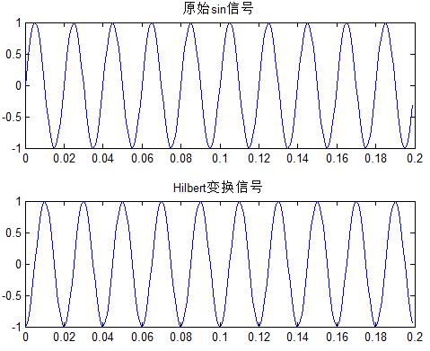
例1:给定一正弦信号,画出其Hilbert信号,直接给代码:
clc
clear all
close all
ts = 0.001;
fs = 1/ts;
N = 200;
f = 50;
k = 0:N-1;
t = k*ts;
% 信号变换
% 结论:sin信号Hilbert变换后为cos信号
y = sin(2*pi*f*t);
yh = hilbert(y);    % matlab函数得到信号是合成的复信号
yi = imag(yh);      % 虚部为书上定义的Hilbert变换
figure
subplot(211)
plot(t, y)
title('原始sin信号')
subplot(212)
plot(t, yi)
title('Hilbert变换信号')
ylim([-1,1])
对应效果图:
例2:已知信号$x(t) = (1 + 0.5\cos (2\pi 5t))\cos (2\pi 50t + 0.5\sin (2\pi 10t))$,求解该信号的包络和瞬时频率。
分析:根据解包络原理知:
信号包络:$(1 + 0.5\cos (2\pi 5t))$
瞬时频率:$\frac{2\pi 50t + 0.5\sin (2\pi 10t)}{2\pi}$
那么问题来了,实际情况是:我们只知道$x(t)$的结果,而不知道其具体表达形式,这个时候,上文的推导就起了作用:可以借助信号的Hilbert变换,从而求解信号的包络和瞬时频率。
对应代码:
clear all; clc; close all;

fs=400;                                 % 采样频率
N=400;                                  % 数据长度
n=0:1:N-1;
dt=1/fs;
t=n*dt;                                 % 时间序列
A=0.5;                                  % 相位调制幅值
x=(1+0.5*cos(2*pi*5*t)).*cos(2*pi*50*t+A*sin(2*pi*10*t));  % 信号序列
z=hilbert(x');                          % 希尔伯特变换
a=abs(z);                               % 包络线
fnor=instfreq(z);                       % 瞬时频率
fnor=[fnor(1); fnor; fnor(end)];        % 瞬时频率补齐
% 作图
pos = get(gcf,'Position');
set(gcf,'Position',[pos(1), pos(2)-100,pos(3),pos(4)]);
subplot 211; plot(t,x,'k'); hold on;
plot(t,a,'r--','linewidth',2);
title('包络线'); ylabel('幅值'); xlabel(['时间/s' 10 '(a)']);
ylim([-2,2]);
subplot 212; plot(t,fnor*fs,'k'); ylim([43 57]);
title('瞬时频率'); ylabel('频率/Hz');  xlabel(['时间/s' 10 '(b)']);
其中instfreq为时频工具包的代码,可能有的朋友没有该代码,这里给出其程序:
function [fnormhat,t]=instfreq(x,t,L,trace);
%INSTFREQ Instantaneous frequency estimation.
%	[FNORMHAT,T]=INSTFREQ(X,T,L,TRACE) computes the instantaneous
%	frequency of the analytic signal X at time instant(s) T, using the
%	trapezoidal integration rule.
%	The result FNORMHAT lies between 0.0 and 0.5.
%
%	X : Analytic signal to be analyzed.
%	T : Time instants	        (default : 2:length(X)-1).
%	L : If L=1, computes the (normalized) instantaneous frequency
%	    of the signal X defined as angle(X(T+1)*conj(X(T-1)) ;
%	    if L>1, computes a Maximum Likelihood estimation of the
%	    instantaneous frequency of the deterministic part of the signal
%	    blurried in a white gaussian noise.
%	    L must be an integer       	(default : 1).
%	TRACE : if nonzero, the progression of the algorithm is shown
%	                                (default : 0).
%	FNORMHAT : Output (normalized) instantaneous frequency.
%	T : Time instants.
%
%	Examples :
%	 x=fmsin(70,0.05,0.35,25); [instf,t]=instfreq(x); plot(t,instf)
%	 N=64; SNR=10.0; L=4; t=L+1:N-L; x=fmsin(N,0.05,0.35,40);
%	 sig=sigmerge(x,hilbert(randn(N,1)),SNR);
%	 plotifl(t,[instfreq(sig,t,L),instfreq(x,t)]); grid;
%	 title ('theoretical and estimated instantaneous frequencies');
%
%	See also  KAYTTH, SGRPDLAY.

%	F. Auger, March 1994, July 1995.
%	Copyright (c) 1996 by CNRS (France).
%
%	------------------- CONFIDENTIAL PROGRAM --------------------
%	This program can not be used without the authorization of its
%	author(s). For any comment or bug report, please send e-mail to
%	f.auger@ieee.org

if (nargin == 0),
 error('At least one parameter required');
end;
[xrow,xcol] = size(x);
if (xcol~=1),
 error('X must have only one column');
end

if (nargin == 1),
 t=2:xrow-1; L=1; trace=0.0;
elseif (nargin == 2),
 L = 1; trace=0.0;
elseif (nargin == 3),
 trace=0.0;
end;

if L<1,
 error('L must be >=1');
end
[trow,tcol] = size(t);
if (trow~=1),
 error('T must have only one row');
end;

if (L==1),
 if any(t==1)|any(t==xrow),
  error('T can not be equal to 1 neither to the last element of X');
 else
  fnormhat=0.5*(angle(-x(t+1).*conj(x(t-1)))+pi)/(2*pi);
 end;
else
 H=kaytth(L);
 if any(t<=L)|any(t+L>xrow),
  error('The relation L<T<=length(X)-L must be satisfied');
 else
  for icol=1:tcol,
   if trace, disprog(icol,tcol,10); end;
   ti = t(icol); tau = 0:L;
   R = x(ti+tau).*conj(x(ti-tau));
   M4 = R(2:L+1).*conj(R(1:L));

   diff=2e-6;
   tetapred = H * (unwrap(angle(-M4))+pi);
   while tetapred<0.0 , tetapred=tetapred+(2*pi); end;
   while tetapred>2*pi, tetapred=tetapred-(2*pi); end;
   iter = 1;
   while (diff > 1e-6)&(iter<50),
    M4bis=M4 .* exp(-j*2.0*tetapred);
    teta = H * (unwrap(angle(M4bis))+2.0*tetapred);
    while teta<0.0 , teta=(2*pi)+teta; end;
    while teta>2*pi, teta=teta-(2*pi); end;
    diff=abs(teta-tetapred);
    tetapred=teta; iter=iter+1;
   end;
   fnormhat(icol,1)=teta/(2*pi);
  end;
 end;
end;
对应的结果图为:
可以看到信号的包络、瞬时频率,均已完成求解。
例3:例2中信号包络为规则的正弦函数,此处给定任意形式的包络(以指数形式为例),并利用Hilbert求解包络以及瞬时频率,并给出对应的Hilbert谱。
程序:
clc
clear all
close all
ts = 0.001;
fs = 1/ts;
N = 200;
k = 0:N-1;
t = k*ts;
% 原始信号
f1 = 10;
f2 = 70;
% a = cos(2*pi*f1*t);       % 包络1
a = 2 + exp(0.2*f1*t);     % 包络2
% a = 1./(1+t.^2*50);       % 包络3
m = sin(2*pi*f2*t);         % 调制信号
y = a.*m;  % 信号调制
figure
subplot(241)
plot(t, a)
title('包络')
subplot(242)
plot(t, m)
title('调制信号')
subplot(243)
plot(t, y)
title('调制结果')
% 包络分析
% 结论:Hilbert变换可以有效提取包络、高频调制信号的频率等
yh = hilbert(y);
aabs = abs(yh);                 % 包络的绝对值
aangle = unwrap(angle(yh));     % 包络的相位
af = diff(aangle)/2/pi;         % 包络的瞬时频率,差分代替微分计算
% NFFT = 2^nextpow2(N);
NFFT = 2^nextpow2(1024*4);      % 改善栅栏效应
f = fs*linspace(0,1,NFFT);
YH = fft(yh, NFFT)/N;           % Hilbert变换复信号的频谱
A = fft(aabs, NFFT)/N;          % 包络的频谱
subplot(245)
plot(t, aabs,'r', t, a)
title('包络的绝对值')
legend('包络分析结果', '真实包络')
subplot(246)
plot(t, aangle)
title('调制信号的相位')
subplot(247)
plot(t(1:end-1), af*fs)
title('调制信号的瞬时频率')
subplot(244)
plot(f,abs(YH))
title('原始信号的Hilbert谱')
xlabel('频率f (Hz)')
ylabel('|YH(f)|')
subplot(248)
plot(f,abs(A))
title('包络的频谱')
xlabel('频率f (Hz)')
ylabel('|A(f)|')
对应结果图:
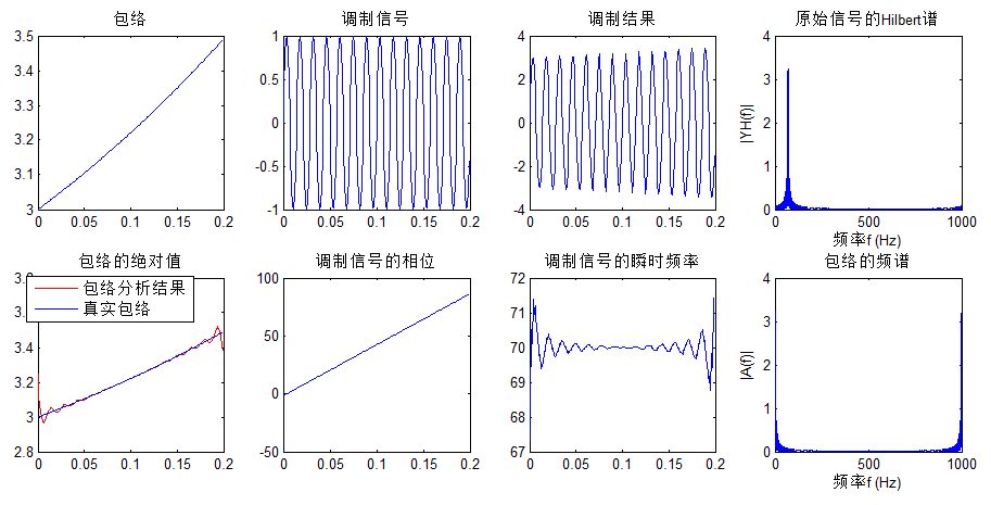
从结果可以观察,出了边界误差较大,结果值符合预期。对于边界效应的分析,见扩展阅读部分。注意:此处瞬时频率求解,没有用instfreq函数,扩展阅读部分对该函数作进一步讨论。
三、扩展阅读
A-瞬时频率求解方法对比
对于离散数据,通常都是用差分代替微分,因此瞬时频率也可根据概念直接求解。此处对比分析两种求解瞬时频率的方法,给出代码:
clc
clear all
close all
ts = 0.001;
fs = 1/ts;
N = 200;
k = 0:N-1;
t = k*ts;
% 原始信号
f1 = 10;
f2 = 70;
% a = cos(2*pi*f1*t);       % 包络1
a = 2 + exp(0.2*f1*t);     % 包络2
% a = 1./(1+t.^2*50);       % 包络3
m = sin(2*pi*f2*t);         % 调制信号
y = a.*m;  % 信号调制
figure
yh = hilbert(y);
aangle = unwrap(angle(yh));     % 包络的相位
af1 = diff(aangle)/2/pi;         % 包络的瞬时频率,差分代替微分计算
af1 = [af1(1),af1];
subplot 211
plot(t, af1*fs);hold on;
plot(t,70*ones(1,length(t)),'r--','linewidth',2);
title('直接求解调制信号的瞬时频率');
legend('频率估值','真实值','location','best');
subplot 212
af2 = instfreq(yh.').';
af2 = [af2(1),af2,af2(end)];
plot(t, af2*fs);hold on;
plot(t,70*ones(1,length(t)),'r--','linewidth',2);
title('instfreq求解调制信号的瞬时频率');
legend('频率估值','真实值','location','best');
结果图:
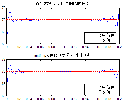
可以看出,两种方式结果近似,但instfreq的结果更为平滑一些。
B-端点效应分析
对于任意包络,求解信号的包络以及瞬时频率,容易出现端点误差较大的情况,该现象主要基于信号中的Gibbs现象,限于篇幅,拟为此单独写一篇文章,具体请参考:Hilbert端点效应分析。
C-VMD、EMD
Hilbert经典应用总绕不开HHT(Hilbert Huang),HHT基于EMD,近年来又出现了VMD分解,拟为此同样写一篇文章,略说一二心得,具体参考:EMD、VMD的一点小思考。
D-解包络方法
需要认识到,Hilbert不是解包络的唯一途径,低通滤波(LPF)等方式一样可以达到该效果,只不过截止频率需要调参。
给出一个Hilbert、低通滤波解包络的代码:
function y=envelope(signal,Fs)

%Example:
%   load('s4.mat');
%   signal=s4;
%   Fs=12000;
%   envelope(signal,Fs);
clc;
close all;

%Normal FFT
y=signal;
figure();
N=2*2048;T=N/Fs;
sig_f=abs(fft(y(1:N)',N));
sig_n=sig_f/(norm(sig_f));
freq_s=(0:N-1)/T;
subplot 311
plot(freq_s(2:250),sig_n(2:250));title('FFT of Original Signal');


%Envelope Detection based on Low pass filter and then FFT
[a,b]=butter(2,0.1);%butterworth Filter of 2 poles and Wn=0.1
%sig_abs=abs(signal); % Can be used instead of squaring, then filtering and
%then taking square root
sig_sq=2*signal.*signal;% squaring for rectifing
%gain of 2 for maintianing the same energy in the output
y_sq = filter(a,b,sig_sq); %applying LPF
y=sqrt(y_sq);%taking Square root
%advantages of taking square and then Square root rather than abs, brings
%out some hidden information more efficiently
N=2*2048;T=N/Fs;
sig_f=abs(fft(y(1:N)',N));
sig_n=sig_f/(norm(sig_f));
freq_s=(0:N-1)/T;
subplot 312
plot(freq_s(2:250),sig_n(2:250));title('Envelope Detection: LPF Method');


%Envelope Detection based on Hilbert Transform and then FFT
analy=hilbert(signal);
y=abs(analy);
N=2*2048;T=N/Fs;
sig_f=abs(fft(y(1:N)',N));
sig_n=sig_f/(norm(sig_f));
freq_s=(0:N-1)/T;
subplot 313
plot(freq_s(2:250),sig_n(2:250));title('Envelope Detection : Hilbert Transform')
结果图:
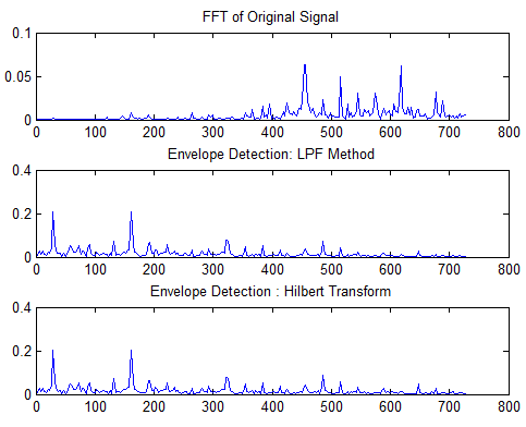
效果是不是也不错?
Hilbert硬件实现思路:
思路1(时域处理):借助MATLAB fdatool实现,Hilbert transform,导出滤波器系数
思路2(频域处理):
参考:
了凡春秋:http://blog.sina.com.cn/s/blog_6163bdeb0102e1wv.html#cmt_3294265

