Quantum Computer Science

Quantum Foundation

Formalism of Quantum Mechanics

State

\(\Leftrightarrow\) vector \(|\psi\rangle\).

Observable

\(\Leftrightarrow\) Hermitian operator \(A=A^*\).

Evolution

Schrödinger's Equation:

\[i\hslash\frac{\partial |\psi\rangle}{\partial t}=\hat{H}|\psi\rangle. \]

If \(\hat{H}\) is time-independent,

\[|\psi(t)\rangle=e^{-\frac{i\hat{H}(t-t_0)}{\hslash}}|\psi(t_0)\rangle=U(t,t_0)|\psi(t_0)\rangle. \]

Evolution operator \(U\) is unitary and norm-preserving.

Measurement

Measure an observable \(A\) under initial state \(|\psi\rangle\), the final state is collapsed to an eigenstates \(|\lambda_i\rangle\) of \(A\) w.p. \(p_i=|\langle\lambda_i|\psi\rangle|^2\).

Quantum no-cloning theorem

Cloning: unitary operator \(U\) s.t. \(U(|\psi\rangle_A|0\rangle_B)=|\psi\rangle_A|\psi\rangle_B.\)

Take two particular states \(|\psi_1\rangle, |\psi_2\rangle\), with \(\langle \psi_1 | \psi_2 \rangle \neq 0,1\), then

\[U|\psi_1\rangle |0\rangle_B = |\psi_1\rangle_A|\psi_1\rangle_B \]

\[U|\psi_2\rangle |0\rangle_B = |\psi_2\rangle_A|\psi_2\rangle_B \]

Inner product of above equations

\[\langle \psi_1|\psi_2 \rangle = \langle \psi_1|\psi_2 \rangle^2 \Rightarrow \langle \psi_1|\psi_2 \rangle = 0, 1 \]

contradiction.

State distinguishability

perfect distinguishable \(\Leftrightarrow\) orthogonal

Quantum Systems

Finite-dim quantum system

A Hilbert space with basis states \(|e_0\rangle,...,|e_{d-1}\rangle\).

The case of \(d=2\) is particularly important. (\(2\)-D system: qubit, spin)

Basis states: \(|0\rangle=\begin{pmatrix}1\\0\end{pmatrix}, |1\rangle=\begin{pmatrix}0\\1\end{pmatrix}\).

For arbitary state (\(|c_0|^2+|c_1|^2=1\))

\[\begin{align*} |\psi\rangle=&\ c_0|0\rangle+c_1|1\rangle=\begin{pmatrix}c_0\\c_1\end{pmatrix}\\ =&\ e^{ir}\left(\cos\left(\frac{\theta}{2}\right)|0\rangle+e^{i\phi}\sin\left(\frac{\theta}{2}\right)|1\rangle\right) \end{align*} \]

Geometric representation: \(\Omega = (\theta,\phi)\)

• \(r\): Globe phase (not important)
• \(\phi\): relative phase
• \(\theta\): angle

Basis operators: Identity matrix and Pauli matrices.

Any operator can be expressed as \(A = r_1I + r_2\sigma_x+r_3\sigma_y+r_4\sigma_y\).

Spin operator: \(\vec{S}=\frac{\hslash}{2}\vec{\sigma}.\)

Eigenvalues of Pauli matrix: \(\pm 1\).

Eigenstates:

\[\sigma_z: \; |0\rangle, |1\rangle \]

\[\sigma_x: \; \frac{|0\rangle + |1\rangle}{\sqrt{2}}, \frac{|0\rangle - |1\rangle}{\sqrt{2}} \]

\[\sigma_y: \; \frac{|0\rangle + i|1\rangle}{\sqrt{2}}, \frac{|0\rangle - i|1\rangle}{\sqrt{2}} \]

Continuous-variable systems:

\(\hat{x}\) (coordinate) and \(\hat{p}\) (momentum)

Spectro-decomposition:

\[\begin{cases} \hat{x}=\int x|x\rangle\langle x|\mathrm{d}x\\ \hat{p}=\int p|p\rangle\langle p|\mathrm{d}p \end{cases}\]

\(|x\rangle\) are eigenspaces s.t.

\[\langle x|x'\rangle=\delta(x-x'), \]

where $$\delta(x)\equiv\frac{1}{2\pi}\int e^{ikx}\mathrm{d}x.$$

This gives completeness:

\[\int x|x\rangle\langle x|\mathrm{d}x=\hat{I}. \]

The momentum of a particle is described by a plane wave with \(k=\frac{p}{\hslash}\):

\[|p\rangle=\frac{1}{\sqrt{2\pi\hslash}}e^\frac{ipx}{\hslash}|\rangle. \]

Thus

\[\langle x|p\rangle=\langle p|x\rangle^*=\frac{1}{\sqrt{2\pi\hslash}}e^\frac{ipx}{\hslash}. \]

Consider the representations of any state \(\psi\) in the coordinate basis and momentum basis:

\[\psi(x)\equiv\langle x|\psi\rangle, \]

\[\phi(p)\equiv\langle p|\psi\rangle. \]

Then we have

\[\phi(p)=\langle p|\psi\rangle=\int\langle p|x\rangle\langle x|\psi\rangle\mathrm{d}x=\int \psi(x)\frac{e^{-\frac{ipx}{\hslash}}}{\sqrt{2\pi\hslash}}\mathrm{d}x. \]

Similarly,

\[\psi(x)=\int \phi(p)\frac{e^{\frac{ipx}{\hslash}}}{\sqrt{2\pi\hslash}}\mathrm{d}p. \]

Furthermore, we can represent \(\hat{p}\) in the coordinate basis:

\[\begin{align*} \hat{p} = &\ \int p \vert p \rangle \langle p \vert \mathrm{d}p \\ = &\ \int p \vert x \rangle \langle x \vert p \rangle \langle p \vert x' \rangle \langle x'|\mathrm{d}p \mathrm{d}x \mathrm{d}x' \\ = &\ \int p \vert x \rangle \langle x' \vert \frac{e^{ip(x-x')/\hslash}}{2\pi\hslash} \mathrm{d}x \mathrm{d}x' \mathrm{d}p \\ = &\ \int \vert x \rangle \langle x' \vert \left( i\hslash\frac{\mathrm{d}}{\mathrm{d}x'} \frac{e^{ip(x-x')/\hslash}}{2\pi\hslash} \right) \mathrm{d}x \mathrm{d}x' \mathrm{d}p \\ = &\ \int \vert x \rangle \left( -i \hslash \frac{\mathrm{d}}{\mathrm{d}x'} \right) \langle x' \vert \delta(x - x') \mathrm{d}x' \mathrm{d}x \\ = &\ \int \vert x \rangle \left( -i \hslash \frac{\mathrm{d}}{\mathrm{d}x} \right) \langle x \vert \mathrm{d}x \end{align*} \]

Thus $$\hat{p}\Leftrightarrow -i\hslash\frac{\mathrm{d}}{\mathrm{d}x}.$$

Similarly, in the momentum basis,

\[\hat{p}\Leftrightarrow i\hslash\frac{\mathrm{d}}{\mathrm{d}p}. \]

From it, we can calculate that

\[[\hat{x},\hat{p}]=i\hslash. \]

Uncertainty Relation, Schrödinger versus Heisenberg Picture

Uncertainty relations

Def. For any operators \(A\), let \(\langle A\rangle=\langle\psi |A|\psi\rangle\) (for any state \(|\psi\rangle\)) and \(\langle(\Delta A)^2\rangle=\langle A^2\rangle-\langle A\rangle^2,\Delta A=A-\langle A\rangle.\)

Thm. For any two operators \(A\) and \(B\), with \([A,B]\neq 0\),

\[\langle(\Delta A)^2\rangle\langle(\Delta B)^2\rangle\ge\frac{1}{4}|\langle[A,B]\rangle|^2. \]

Ex. Let \(A=\hat{x},B=\hat{p}\) gives $$\langle(\Delta A)^2 \rangle\langle(\Delta B)^2 \rangle\ge\frac{\hslash^2 }{4}.$$
Let \(A=\hat{\sigma_x},B=\hat{\sigma_y}\) gives $$\langle(\Delta A)^2 \rangle\langle(\Delta B)^2 \rangle\ge\langle\hat{\sigma_z}\rangle^2.$$

Evolution in the Schrödinger picture

Schrödinger picture: State evolves, but operator does not.

State evolution follows Schrödinger's equation:

\[i\hbar \frac{\partial}{\partial t} |\psi\rangle = \hat{H} |\psi\rangle \]

For a continuous variable (CV) system,

\[\hat{H}(\hat{x}, \hat{p}) = \frac{\hat{p}^2}{2m} + V(\hat{x}) \]

In the coordinate representation, it gives

\[i \hslash \frac{\partial}{\partial t} \psi(\vec{r}) = \left[ -\frac{\hslash^2}{2m} \nabla_{\vec{r}}^2 + V(\vec{r}) \right] \psi(\vec{r}) \]

In the momentum representation, it gives

\[i \hslash \frac{\partial}{\partial t} \phi(p) = \left[ \frac{p^2}{2m} + V\left( i \hslash \frac{\partial}{\partial p} \right) \right] \phi(p) \]

Evolution in the Heisenberg picture

Heisenberg picture: Operator evolves, but state does not.

Let \(H\) be a time-independent operator s.t.

\[i \hslash \frac{\partial\hat{U}}{\partial t} = H\hat{U} \]

Heisenberg equation:

\[i \hslash \frac{\mathrm{d}A_H}{\mathrm{d}t} = [A_H, H] \]

Dynamics of 2-dimensional systems

2-D Hamiltonian \(H=\hslash(\alpha\hat{I}+\frac{w}{2}\vec{n}\cdot\vec{\sigma})\).

Evolution operator: $$U(t)=e^{-\frac{iHt}{\hslash}} =e^{-i\alpha t} \left(\hat{I}\cos\frac{wt}{2}-i\vec{n}\cdot\vec{\sigma}\sin\frac{wt}{2}\right).$$

Multi-Partite Quantum Systems

Density operator

Def. density operator:

\[\rho=\sum\limits_i p_i|\psi_i\rangle\langle \psi_i|, \]

where \(\sum\limits_i p_i=1.\)

Property of trace: $$tr(AB)=tr(BA),$$$$tr(A+B)=tr(A)+tr(B),$$$$tr(|\psi\rangle\langle \psi|)=\langle \psi|\psi\rangle,$$$$tr(A|\psi\rangle\langle \psi|)=\langle \psi|A|\psi\rangle,$$$$tr(A)=\sum\limits_i\langle\psi_i|A|\psi_i\rangle.$$

Def [partial trace]. $$tr_2(B_{12})=\sum\limits_i\langle\psi_{2i}|B_{12}|\psi_{2i}\rangle.$$

\[\langle A_1\rangle=_{12}\langle\psi|A|\psi\rangle_{12}=tr_1(Atr_2(|\psi\rangle_{12 12}\langle\psi|))=tr_1(\rho_1A_1), \]

where \(\rho_1=tr_2(|\psi\rangle_{12 12}\langle\psi|)\).

Prop. 1 [Characterization Theorem] Any Hermitian operator \(\rho\) is a density operator iff \(tr(\rho)=1\) and \(\rho\) has non-negative eigenvalues.

Prop. 2 [Pure state criterion] \(tr(\rho^2)\le 1\). \(tr(\rho^2)=1\) iff \(\rho\) is a pure state, with \(\rho=|\psi\rangle\langle\psi|\).

Entanglement and entropy

Def. [entanglement] For pure state \(|\psi\rangle_{AB}\), if \(|\psi\rangle_{AB}\neq |\phi_A\rangle_A\otimes|\phi_B\rangle_B\), it is entangled.

Def. [Von-Neumann entropy] \(S(\rho)=-tr(\rho\log\rho)=-\sum_i\lambda_i\log\lambda_i,\)where \(\lambda_i\) are eigenvalues of \(\rho\).

Prop.

\(S(U\rho U^\dagger)\), for unitary operator \(U\).
\(S(\ket{\psi}\bra{\psi})=0.\)
\(S(\lambda_1\rho_1+\lambda_2\rho_2)\ge \lambda_1S(\rho_1)+\lambda_2S(\rho_2).\)
Subadditivity: \(S(\rho_{AB})\le S(\rho_A)+S(\rho_B),\) equality holds when \(\rho_{ab}=\rho_a\otimes\rho_b.\)
Strong subadditivity: \(S(\rho_{ABC})+S(\rho_B)\le S(\rho_{AB})+S(\rho_{BC}).\)

Entanglement measure: entanglement of a bi-partite pure state \(\ket{\psi}_{AB}\) is measured by $$E(\ket{\psi}_{AB})=S(\rho_A)=S(\rho_B).$$

Schmidt decomposition

Thm. For any pure state \(\ket{\psi}_{AB}\), there exists a basis \(\{\ket{i}_A\}\) s.t.

\[\ket{\psi}_{AB}=\sum_i\sqrt{p_i}\ket{i}_A\ket{\mu_i}_B, \]

with \(\sum_i p_i=1.\) \(p_i\) is called Schmidt number.

Pf. Assume

\[\ket{\psi}_{AB}=\sum\limits_{i\mu} a_{i\mu}\ket{i}_A\ket{\mu}_B=\sum\limits_i\ket{i}_A\ket{\tilde{i}}_B \]

with

\[\ket{\tilde{i}}_B\equiv\sum\limits_\mu a_{i\mu}\ket{\mu}_B. \]

Then

\[\rho_A=\text{tr}_B(\ket{\psi}_{AB}\bra{\psi})=\text{tr}_B(\sum\limits_{ij}\ket{i}_A\ket{\tilde{i}}_{B A}\bra{j}_B\bra{\tilde{j}})=\sum_{ij}\ket{i}_{AA}\bra{j}_B\braket{\tilde{j}|\tilde{i}}_{B}. \]

Assume \(\ket{i}_A\) to be the eigenbasis of \(\rho_A\), that is, $$\rho_A=\sum\limits_i p_i\ket{i}_A \bra{i}.$$

Thus $$\langle\tilde{j}|\tilde{i}\rangle_{B}=p_i\delta_{ij}.$$

Let \(\ket{\mu_i}\equiv\frac{1}{\sqrt{p_i}}\ket{\tilde{i}}\), by above analysis, \(\ket{\mu_i}\) is orthonormal, and satisfies

\[\ket{\psi}_{AB}=\sum_i\sqrt{p_i}\ket{i}_A\ket{\mu_i}_B. \]

Prop.

\(\rho_B=\sum\limits_ip_i\ket{\mu_i}_B\bra{\mu_i}.\)
purification: any mixed state \(\rho_A\) can be written in the form

\[\rho_A=\text{tr}_B(\ket{\psi}_{AB}\bra{\psi}), \]

\(\ket{\psi}_{AB}\) is called purification of \(\rho_A\) and \(\dim(H_B)\le \dim(H_A)\)

Generalized Evolution: Superoperators

Assume that in initial,

\[\rho_{AB}=\rho_A\otimes\ket{E}_B\bra{E} \]

(No entanglement between \(A\) and \(B\)). Then after evolution,

\[\rho'_{AB}=U_{AB}(\rho_A\otimes\ket{E}_B\bra{E})U^\dagger_{AB}. \]

Thus

\[\rho'_A=\text{tr}_B(\rho'_{AB})=\sum\limits_\mu\bra{\mu}_BU_{AB}(\rho_A\otimes\ket{E}_B\bra{E})U^\dagger_{AB}\ket{\mu}_B =\sum\limits_\mu M_\mu\rho_AM^\dagger_\mu \]

where

\[M_\mu\equiv\bra{\mu}_BU_{AB}\ket{\mu}_B \]

is an operator acting on \(H_A\).

Prop. $$\sum\limits_{\mu}M^\dagger_\mu M_\mu=I_A.$$

A mapping \(\hat{\$}:\rho\rightarrow \rho'\) is a superoperator, it might have following properties:

(0). linear
(1). hermiticity-preserving: \(\rho'\) hermitian if \(\rho\) is
(2). trace-preserving: \(\text{tr}(\rho')=1\) if \(\text{tr}(\rho)=1\)
(3). positive: \(\rho'\) is non-negative if \(\rho\) is positive
(3'). completely positive: any extensive \(\hat{\$}\otimes I_B\) is positive

Thm. [Kraus's Theorem] Any superoperator satisfying \((0),(1),(2),(3')\) has an operator-sum representation, i.e.

\[\hat{\$_A}(\rho_A)=\sum\limits_\mu M_\mu\rho_AM^\dagger_\mu \]

with

\[\sum\limits_\mu M^\dagger_\mu M_\mu=I_A. \]

Rem. At most \(\dim(H_A)^2\) of \(M_\mu\).

Assume \(\delta t\) is small,

\[\rho(t+\delta t)=\rho(t)+\delta t\dot{\rho}. \]

On the other hand, $$\rho(t+\delta t)=\hat{$}(\rho(t))=\sum\limits_{\mu}M_\mu\rho(t)M^\dagger_\mu.$$

One \(M_\mu\) must be close to \(I\), let \(M_0=I+\delta t(-iH+K)\) and \(M_\mu=L_\mu \sqrt{\delta t}\) for \(\mu\neq 0\). Then

\[I=\sum\limits_\mu M_\mu^\dagger M_\mu=M_0^\dagger M_0+\sum\limits_{\mu\neq 0} M_\mu^\dagger M_\mu=I+(2K+\sum\limits_{\mu}L^\dagger_\mu L_\mu)\delta t \]

Thus

\[K=-\frac{1}{2}\sum\limits_{\mu}L^\dagger_\mu L_\mu. \]

Substituting it gives:

Thm. [Master Equation]

\[\dot{\rho}=\frac{\rho(t+\delta t)-\rho(t)}{\delta t}= -i[H, \rho] + \sum_\mu \left( L_\mu \rho L_\mu^\dagger - \frac{1}{2} L_\mu^\dagger L_\mu \rho - \frac{1}{2} \rho L_\mu^\dagger L_\mu \right) \]

Also we have the inverse theoerm for Kraus's Theorem.

Thm. Any evolution \(\hat{\$}\) on density operator \(\rho_A\) with \(\hat{\$}(\rho_A)=\sum\limits_\mu M_\mu\rho_AM^\dagger_\mu\) can be implemented with a unitary evolution \(U_{AB}\) in the extended space \(H_A\otimes H_B\) with

\[\text{tr}_B[U_{AB}(\rho_A\otimes \ket{E}_B\bra{E})U^\dagger_{AB}]=\sum\limits_\mu M_\mu\rho_AM^\dagger_\mu. \]

Ex.

1. Depolarizing channel

   For a qubit state

   \[p\begin{cases} \text{a bit flip } \sigma_x = X \\ \text{a phase flip } \sigma_z = Z \\ \text{a bit-phase flip } \sigma_y = Y = iXZ \end{cases}\text{ error}. \]

   Krause Rep.

   \[\rho\to\hat{\$}(\rho)=\sum\limits_{i=0,1,2,3}M_\mu\rho M_{\mu}^\dagger, \]

   with \(M_0 = \sqrt{1-p}I, \quad M_1 = \sqrt{\frac{p}{3}}X, \quad M_2 = \sqrt{\frac{p}{3}}Y, \quad M_3 = \sqrt{\frac{p}{3}}Z\).

   Substituting gives

   \[\rho' = (1 - p)\rho + \frac{p}{3} (X\rho X + Y\rho Y + Z\rho Z). \]

   In Bloch Sphere Rep.

   Assume \(\rho = \frac{1}{2}(I + \vec{p} \cdot \vec{\sigma})\),

   \[\rho' = \frac{1}{2}(I + \vec{p}' \cdot \vec{\sigma}),\text{with }\vec{p}' = \left(1 - \frac{4}{3}p \right) \vec{p} \]

   It becomes complete randomized when \(p=\frac{3}{4}\).

2. Phase-damping channel

   \[\begin{cases}1-p & \text{no error} & I\\p & \text{a phase flip error} & \sigma_z=Z\end{cases} \]

   Krause operator \(M_0=\sqrt{1-p}I,M_1=\sqrt{p}Z\).

   \[\hat{\$}(\rho)=(1-p)\rho+pZ\rho Z. \]

3. Amplitude-damping channel

   \[\begin{cases}\ket{0}_A\ket{E}\to\ket{0}_A\ket{E}\\ \ket{1}_A\ket{E}\to\sqrt{1-p}\ket{1}_A\ket{E}+\sqrt{p}\ket{0}_A\ket{E'}\end{cases} \]

   Krause operator \(M_0 = \begin{pmatrix} 1 & 0 \\ \sqrt{1 - p} & 0 \end{pmatrix}, M_1 = \begin{pmatrix} 0 & \sqrt{p} \\ 0 & 0 \end{pmatrix}\).

   \[\rho \rightarrow \hat{\$}(\rho) = \begin{pmatrix} \rho_{00} + p \rho_{11} & \sqrt{1 - p} \rho_{01} \\ \sqrt{1 - p} \rho_{10} & (1 - p) \rho_{11} \end{pmatrix} \]

Generalized Measurements: POVM

Von Neumann measurement

Projectors \(\{E_i\}\) satisfies \(\begin{cases}E_iE_j=\delta_{ij}E_i\\\sum_iE_i=I\end{cases}\) can be used to describle an observable.

Then \(\rho\rightarrow \rho'=E_i\rho E_i\) with \(p_i=\text{tr}(E_i\rho).\)

POVM

Extension to composite system. What is its form in reduced system \(A\) when measure \(AB\)?

Assume \(\rho_{AB}=\rho_A\otimes\rho_B\). The probability of \(\rho'_A=\text{tr}_B(E_i\rho_{AB}E_i)\) is

\[p_i=\text{tr}_{AB}(E_i\rho_{AB})=\text{tr}_A(\rho_A\text{tr}_B(E_i\rho_B))=\text{tr}_A(\rho_AF_i) \]

where \(F_i=\text{tr}_{B}(E_i\rho_B)\).

Properties of \(F_i\):

1. Hermitian \(F_i^\dagger=\text{tr}_B(\rho^\dagger_BE_i^\dagger)=F_i\)

2. Positive, for any state \(\ket{\phi}_A\), let \(\rho_A=\ket{\phi}_A\bra{\phi}\),

   \[\braket{\phi|F_i|\phi}_A=\text{tr}_A(F_i\rho_A)=\text{tr}_{AB}(E_i\rho_B\otimes\rho_A)\ge 0 \]

   since \(E_i\) is positive.

3. Complete \(\sum_iF_i=\text{tr}_B\left(\sum_iE_i\rho_B\right)=\text{tr}_B(I_{AB}\rho_B)=I_A\).

Def. A set of \(\{F_i\}\) with properties 1-3 is a POVM.

Rem. In general,

1. \(F_iF_j\neq\delta_{ij}F_i\).
2. no simple describe of states after POVM.

Inverse (Neumark) theorem

Thm. Any POVM \(\{F_i\}\) in \(H_A\) can be implemented with a projective measurement \(\{E_i\}\) in extended space \(H_A\otimes H_B\) with the same probability for outcomes, i.e.,

\[\text{tr}(F_i\rho_A)=p_i=\text{tr}_B(E_i\rho_A\otimes \ket{E}\bra{E}). \]

Quantum Entanglement

Entanglement of Pure States and Von-Neumann Entropy

Def. \(\ket{\psi}_{AB}\) is entangled if \(\ket{\psi}_{AB}\) can not be written as a product state \(\ket{\psi}_{AB}=\ket{\phi_1}_A\otimes\ket{\phi_2}_B.\)

Def. \(S(\rho_A)=-\text{tr}(\rho_A\log\rho_A)=-\sum_i\lambda_i\log \lambda_i.\)

We can see that

\[\begin{cases}S(\rho_A)=0 & \text{if }\rho_A\text{ is a pure state}\\S(\rho_A)=1 & \text{if}\rho_A=\frac{1}{2}I\end{cases} \]

If \(\rho\) has \(D\) non-vanishing eigenvalues, \(S(\rho)\le \log D.\)

Def. For pure states, \(E(\ket{\psi}_{AB})=S(\rho_A)=S(\rho_B)\).

LOCC (𝐿𝑜𝑐𝑎𝑙 𝑜𝑝𝑒𝑟𝑎𝑡𝑖𝑜𝑛, 𝐶𝑙𝑎𝑠𝑠𝑖𝑐𝑎𝑙 𝑐𝑜𝑚𝑚𝑢𝑛𝑖𝑐𝑎𝑡𝑖𝑜𝑛𝑠) does not increase entanglement!

Def. Entanglement of formation: $$E_F(\ket{\psi}{AB})=\frac{k{\min}}{n}$$, where \(k_{\min}\) is the least number of \(\ket{\phi^+}_{AB}\) required to prepare \(n\) copies of \(\ket{\psi}_{AB}\) through LOCC.

Def. Entanglement of distillation: \(E_D(\ket{\psi}_{AB})=\frac{k_{\max}}{n}\), where \(k_{\min}\) is the maximum number of \(\ket{\phi^+}_{AB}\) that can be distilled from \(n\) copies of \(\ket{\psi}_{AB}\) through LOCC.

Thm. \(E_D\le E_F\).

Thm. For any bi-partite pure states,

\[E_D(\ket{\psi}_{AB})=S(\rho_A)= E_F(\ket{\psi}_{AB}). \]

Entanglement Measures For Mixed States

Def. A bi-partite (mixed) state is called entangled (inseparable) iff it cannot be written in the form \(\rho_{AB}=\sum_ip_i\rho_{iA}\otimes\rho_{iB}\).

Rem. With LOCC, one can prepare any separable state.

Thm. Partial transpose (Peres – Horodecki) criteria: For any separable state \(\rho_{AB}\), the partial transpose \(\rho_{AB}^{T_B}\) is positive. The positivity of \(\rho_{AB}^{T_B}\) is also a necessary and sufficient condition for separability of \(\rho_{AB}\) for \(2\times 3\)−dim, and \(2\times 2\)−dim systems. (Not true for \(3\times 3\))

General criteria for entanglement measures: E

1. \(E(\rho_{AB})=0\) iff \(\rho_{AB}\) is separable.
2. \(E(U_A\otimes U_B\rho_{AB}U_A^\dagger\otimes U_B^\dagger)=E(\rho_{AB})\).
3. \(E(\rho_{AB})\) should be non-increasing under LOCC (entanglement monotone)
4. Reduce to Von-Neumann entropy for pure states

Def. For \(\rho_{AB}=\sum_ip_i\ket{\psi_i}_{AB}\bra{\psi_i},\) $$E_C(\rho_{AB})=\min\limits_{\text{ensemble decompositions}}\sum_i p_iE(\ket{\psi_i}_{AB}).$$

Wootters’ formula:

Def. \(\tilde{\rho}_{AB} = (Y_A \otimes Y_B) \rho_{AB}^* (Y_A \otimes Y_B) \quad (Y = \sigma_y)\)

\[R = \sqrt{\rho_{AB} \tilde{\rho}_{AB} \rho_{AB}} \]

\(tr(R)\): generalization of fidelity \(\langle \psi | \rho | \psi \rangle\), \((\text{tr}(R))^2\): fidelity between \(\rho_{AB}\) and \(\tilde{\rho}_{AB}\)

The eigenvalues of \(R\) in decreasing order \(\lambda_1, \lambda_2, \lambda_3, \lambda_4\)

Def. "Concurrence" \(C(\rho_{AB}) = \max \{ 0, \lambda_1 - \lambda_2 - \lambda_3 - \lambda_4 \}\)

A measure of entanglement by itself

\[E_C(\rho_{AB}) = h\left( \frac{1 + \sqrt{1 - C^2(\rho_{AB})}}{2} \right) \]

monotonic in \(C\).

Where the function \(h(x) \equiv -x \log_2 x - (1 - x) \log_2(1 - x)\) (Shannon entropy)

Def. Negativity is the sum of negative eigenvalues of \(\rho_{AB}^{T_B}\), formally,

\[N(\rho_{AB})=\sum_i\frac{|\lambda_i|-\lambda_i}{2} \]

Logarithmic negativity \(LN(\rho_{AB})=\log_2(2N(\rho_{AB})+1)\).

We can show that

\[LN(\rho_{AB})\ge E_D(\rho_{AB}). \]

Typical Entangled States

EPR, Bell, Werner, and Bell diagonal states

EPR (Bell) states for qubits

\[|\psi^\pm \rangle_{AB} = \frac{1}{\sqrt{2}} (|01\rangle \pm |10\rangle) \]

\[|\phi^\pm \rangle_{AB} = \frac{1}{\sqrt{2}} (|00\rangle \pm |11\rangle) \]

Locally equivalent by \(U_A\) (or \(U_B\)). $ E = 1 \text{ ebit} $

Werner state

\[\rho_W = p |\phi^+\rangle\langle\phi^+| + (1 - p) \frac{1}{4} I_{AB} \]

Bell diagonal state

\[\rho_B = p_1 |\psi^+\rangle\langle\psi^+| + p_2 |\psi^-\rangle\langle\psi^-| + p_3 |\phi^+\rangle\langle\phi^+| + p_4 |\phi^-\rangle\langle\phi^-| \]

\[\sum_i p_i = 1 \]

GHZ, W, and Dicke states

GHZ states

\[|GHZ_3 \rangle \equiv \frac{1}{\sqrt{2}} (|000\rangle + |111\rangle) \]

\[|GHZ_N \rangle \equiv \frac{1}{\sqrt{2}} (|0\rangle^{\otimes N} + |1\rangle^{\otimes N}) \]

W states

\[|W_3 \rangle \equiv \frac{1}{\sqrt{2}} (|001\rangle + |010\rangle + |100\rangle) \]

Dicke states

\[\ket{\frac{N}{2}, \frac{n}{2}} \propto (S^+)^n |0\rangle^{\otimes N} \]

where collective spin operator \(S^+=\sum\limits_i\sigma_i^+\). Similar, we have \(S_x,S_y,S_z\). Define \(\vec{S}=(S_x,S_y,S_z)\).

We can show that Dicke states are eigenstates of \(\vec{S}^2\):

\[\vec{S}^2\ket{\frac{N}{2},\frac{n}{2}}=\frac{N}{2}\left(\frac{N}{2}+1\right)\ket{\frac{N}{2},\frac{n}{2}}. \]

Prop.

1. A single copy of \(\ket{GHZ3}\) and \(\ket{W3}\) cannot convert to each other with non-zero probability by LOCC. They are maximally entangled, representing two classes
2. Entanglement of Dicke state \(\ket{N,n}\) increase with \(n\) for \(n\le\frac{N}{2}\).

Cluster, Graph, and stabilizer states

Many-qubit entangled state

\[\ket{\psi}=\sum_{i_1,i_2,...,i_n}C_{i_1,i_2,...,i_n}\ket{i_1,i_2,...,i_n} \]

is hard to express.

Def. Let \(\{A_i\}\) be a set of stabilizers satisfies for any \(i\neq j\),

\[[A_i,A_j]=0. \]

Take \(A_i\) as tenser products of Pauli matrix (Pauli group), e.g., \(A_i=X_1Z_2X_3Z_4,...\)

Its corresponding stabilizer states are the states stabilized by \(A_i\).

Prop.

1. \([X_iZ_j,Z_iX_j]=0\) holds for any dim. (Use \(X_iZ_i=-Z_iX_i\) or \(X_iZ_i=e^{-i\frac{2\pi}{d}}Z_iX_i.\))

2. \(A_i^2=I,\) \(A_i\) has eigenvalues \(\pm 1\).

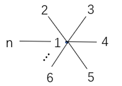
Def. Given a graph \(G\), the corresponding stabilizer state, i.e., co-eigenstates of \(A_i\) with \(+1\) eigenvalue, where \(A_i\) associate with \(i\) qubit is \(A_i=X_i\prod_{j\in N(i)}Z_j\), is a graph state. When the graph is a chain, it's also called cluster state.

Thm. The graph state of \(G\) is

\[\Pi_{(u,v)\in E(G)} CZ_{u,v}\ket{+}^{\otimes n}=\sum\limits_{x\in\{0,1\}^n}(-1)^{\sum\limits_{(u,v)\in E}x_ux_v}\ket{x}. \]

Prop.

1. graph states \(\subset\) stabilized state

2. Any stabilizer states by Pauli group can be written as a graph state.

Ex.

• two qubits:

  \[\begin{cases}X_1Z_2\ket{\psi}=\ket{\psi}\\Z_1X_2\ket{\psi}=\ket{\psi}\end{cases}\Rightarrow\ket{\psi}=(\ket{0}_1(\ket{0}_2+\ket{1}_2)+\ket{1}_1(\ket{0}_2-\ket{1}_2)). \]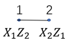

  

• When the dimension is greater than \(2\), its solution (for blossom) becomes local Clifford equivalent to (by \(I_1H_2H_3...H_n\)):

  \[\ket{GHZ_n}=\ket{0}^{\otimes n}+\ket{1}^{\otimes n}. \]

Quantum Nonlocality and Bell’s Inequalities

EPR paradox and hidden variable theory

Einstein and the Copenhagen group debate on quantum nonlocality:

Suppose that \(A\) and \(B\) are spacelike separated systems. Then in a complete description of physical reality an action performed on system \(A\) must not modify the description of system \(B\).

But if \(A\) and \(B\) are entangled, a measurement of \(A\) is performed and a particular outcome is known to have been obtained then the density matrix of \(B\) does change. Therefore by Einstein's criterion the description of a quantum system by a wave function cannot be considered complete.

To interpret this, they proposed the local hidden-variable theory:

Measurement is actually fundamentally deterministic but appears to be probabilistic because some degrees of freedom are not precisely known.

Bell-CHSH inequality

It shows that certain consequences of entanglement in quantum mechanics cannot be reproduced by LHV theory.

Def (Bell-CHSH inequality). Consider \(2\) qubits \(A,B\), with observables \(A_1,A_2,B_1,B_2\). According to LHV, these observables are random variable with values \(\pm1\). Let define a new variable

\[W\equiv (A_1+A_2)B_1-(A_1-A_2)B_2. \]

We can show that \(W=\pm 2\). So \(|\braket{W}|\le 2\) for any probability distribution. This is called Bell-CHSH inequality.

Thm. There exist cases to violate \(|\braket{W}|\le 2\) in QM.

Pf. Take state \(\ket{\psi^-}_{AB}=\frac{1}{\sqrt{2}}(\ket{01}_{AB}-\ket{10}_{AB})\), we have \((\vec{\sigma_A}+\vec{\sigma_B})\ket{\psi^-}_{AB}=0\). Thus for any \(\vec{n},\vec{m}\),

\[\begin{aligned} &_{AB}\langle \psi^- | (\vec{n} \cdot \vec{\sigma}_A)(\vec{m} \cdot \vec{\sigma}_B) | \psi^- \rangle_{AB} \\ =&-_{AB}\langle \psi^- | (\vec{n} \cdot \vec{\sigma}_A)(\vec{m} \cdot \vec{\sigma}_A) | \psi^- \rangle_{AB}\\ = & -\text{tr}_A(\rho_A (\vec{n} \cdot \vec{\sigma}_A)(\vec{m}\cdot\vec{\sigma_A}))\\ = &-\vec{n} \cdot \vec{m}\\ = &-\cos(\theta_{\vec{n}\vec{m}}). \end{aligned} \]

Define

\[\begin{aligned} A_1 &= \vec{n}_1 \cdot \vec{\sigma}_A, \quad B_1 = \vec{m}_1 \cdot \vec{\sigma}_B \\ A_2 &= \vec{n}_2 \cdot \vec{\sigma}_A, \quad B_2 = \vec{m}_2 \cdot \vec{\sigma}_B \end{aligned} \]

the relationship between the vectors is as follows:

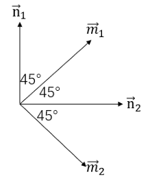
We can calculate that

\[\langle A_1 B_1 \rangle = \langle A_2 B_1 \rangle = \langle A_2 B_2 \rangle = -\frac{1}{\sqrt{2}},\quad\langle A_1 B_2 \rangle = \frac{1}{\sqrt{2}} \]

Immediately,

\[\braket{W} = 2\sqrt{2} >2 \]

which violate the inequality.

Def (sup norm). Define

\[\big||M|\big|=\sup_{\ket{\psi}}\frac{\big||M\ket{\psi}|\big|}{\big|\ket{\psi}|\big|}. \]

Prop.

\[\big||MN|\big|\le \big||M|\big|\big||N|\big|, \]

\[\big||M+N|\big|\le \big||M|\big|+\big||N|\big|. \]

Thm. The maximum violation of Bell’s inequality is \(2\sqrt{2}\).

Pf. Since \(A_i^2=B_i^2=I\) and \([A_i,B_j]=0\), we square

\[W=(A_1+A_2)B_1-(A_1-A_2)B_2 \]

to get

\[W^2=4+[A_1,A_2][B_1,B_2]. \]

Thus

\[\big||W^2|\big|\le 4+4\big||A_1|\big|\big||A_2|\big|\big||B_1|\big|\big||B_2|\big|=8. \]

Immediately,

\[\braket{W}\le 2\sqrt{2}. \]

Thm. For separable state, \(\braket{W}\le 2\).

In fact, it's hard to give a experimental verification due to following loophole:

1. Nonlocality loophole
2. Detector inefficiency loophole

Entanglement-Based Quantum Protocols

Dense coding

Thm. Two classical bits of information can be faithfully transferred by sharing one bit of entanglement and one qubit.

Pf. Assume Alice and Bob share an entangled pair of qubits in the state \(\ket{\phi^+}_{AB}\). Now Alice want to use the quantum channel to send only one qubit to Bob, but carry two bits of information.

By perform one of four possible unitary transformations, Alice transforms \(\ket{\phi^+}_{AB}\) to one of four mutually orthogonal states:

\[\begin{cases} I\ket{\phi^+}_{AB}\to\ket{\phi^+}_{AB}\\ \sigma_x\ket{\phi^+}_{AB}\to\ket{\psi^+}_{AB}\\ \sigma_y\ket{\phi^+}_{AB}\to\ket{\psi^-}_{AB}\\ \sigma_z\ket{\phi^+}_{AB}\to\ket{\phi^-}_{AB}\\ \end{cases} \]

Then, she sends her qubit to Bob. Bob performs an orthogonal collective measurement on the pair that projects onto the maximally entangled basis. The measurement outcome unambiguously distinguishes the four possible actions that Alice could have performed.

Notice that \(\rho_A=\frac{1}{2}I_A\) carries no information. So don't worry that an eavesdropper will intercept the transmitted qubit and decipher the message.

Quantum Key Distribution

Lets suppose that Alice and Bob share a supply of entangled pairs each prepared in the state \(\ket{\psi^-}.\) To establish a shared private key, they may carry out this protocol:

• For each qubit in her his possession, Alice and Bob decide to measure either \(\sigma_x\) or \(\sigma_z\), each with probability \(\frac{1}{2}\).

• After measurements, Alice and Bob publicly announce what observables they measured but do not reveal the outcomes they obtained.

• If they measured along different axes, discarded as Alice and Bob obtained uncorrelated outcomes; If they measured along the same axis, their results though random are perfectly anticorrelated. Hence they have established a shared random key.

• To avoid leakage by entangled with qubits in Eve's possession, they verify the properties \(\braket{\sigma_x^A\sigma_x^B}=-1=\braket{\sigma_z^A\sigma_z^B}\). Alice and Bob can sacrifice a portion of their shared key and publicly compare their measurement outcomes They should find that their results are indeed perfectly correlated.

Quantum Teleportation

Thm. An unknown qubit state can be faithfully transferred by sharing one bit of entanglement and two bits of classical message.

Pf. Assume Alice and Bob share an entangled pair of qubits in the state \(\ket{\phi^+}_{AB}\). Now Alice want to send a qubit \(\ket{\psi}_C=a\ket{0}_C+b\ket{1}_C\) to Bob by exploiting this entangled pair and additional classical message.

We can see that

\[\begin{align*} &\ \ket{\psi}_C\otimes\ket{\phi^+}_{AB}\\ =&\ \frac{1}{\sqrt{2}}(a\ket{0}_C+b\ket{1}_C)\otimes(\ket{00}_{AB}+\ket{11}_{AB})\\ =&\ \frac{1}{\sqrt{2}}\left( a\ket{000}_{CAB} + a\ket{011}_{CAB} + b\ket{100}_{CAB} + b\ket{111}_{CAB} \right)\\ =&\ \frac{1}{2} \Big[ \ket{\phi^+}_{CA}(a\ket{0}_B + b\ket{1}_B) + \ket{\phi^-}_{CA}(a\ket{0}_B - b\ket{1}_B)+ \ket{\psi^+}_{CA}(a\ket{1}_B + b\ket{0}_B) + \ket{\psi^-}_{CA}(a\ket{1}_B - b\ket{0}_B) \Big]\\ =&\ \frac{1}{2} \sum_{i=1}^4 \ket{\text{Bell}_i}_{CA} \otimes (\sigma_i \ket{\psi}_B) \end{align*} \]

Alice measure \(A\) and \(C\) in the bell basis and send the 2 bits outcome to Bob in classical channel. Receiving this information, Bob performs the corresponding operations on \(\ket{\cdot}_B\):

\[\begin{cases} \ket{\phi^+}_{CA}\to I_B\\ \ket{\phi^-}_{CA}\to \sigma_{ZB}\\ \ket{\psi^+}_{CA}\to \sigma_{XB}\\ \ket{\psi^-}_{CA}\to \sigma_{XB}\sigma_{ZB}\\ \end{cases} \]

Now his bit is transformed into a perfect copy of the initial \(\ket{\psi}_C\)!

Quantum Computation

Models of Quantum Computation

Classical circuit model and computation complexity

A classical deterministic computer evaluates a function:

\[f:\{0,1\}^n\to\{0,1\}^m. \]

It's equivalent to solve \(m\) decision problem \(f:\{0,1\}^n\to\{0,1\}.\)

Classical universality: any decision function can be constructed by elementary gates: AND, NOT, OR and COPY.

The evaluation of any such function can be reduced to a sequence of elementary logical operations, the so-called circuit.

For a decision problem, a reasonable measure of hardness is the size of the smallest circuit that computes the corresponding function. Then we define:

\[\mathsf{P}=\{\text{decision problem that admit a polynomial size deterministic circuit family}\}.\\ \mathsf{NP}=\{\text{decision problem that admit a polynomial size nondeterministic circuit family}\}.\\ \]

Quantum computation

Process:

• Input: Pure state \(\ket{\psi_{in}}\) or mixed-state \(\rho_{in}\), the state must be prepared to \(\ket{0}^{\otimes n}\).

• Operation: Unitary operation \(U\) or superoperator \(\$\).

• Output: Applying operation on the input gives \(\ket{\psi_{out}}\) or \(\rho_{out}\).

• Measurement: Projection \(M\) or POVM \(\{F_i\}\). Do it in \(z\)-basis.

We need ancilla to do this in extended space, ancilla is prepared to \(\ket{0}\).

Quantum Gates

Elementary quantum gates

Single qubit gates

A single qubit gate is described by four real parameters:

\[U(\alpha,\beta,\phi,\theta)=e^{i\alpha}\begin{bmatrix}\cos\theta & -\sin\theta e^{i\phi}\\\sin\theta e^{-i\phi} & \cos\theta\end{bmatrix}\begin{bmatrix}1 & 0\\0 & e^{i\beta}\end{bmatrix}. \]

• Pauli gate: \(X=\begin{bmatrix}0 & 1\\1 & 0\end{bmatrix},Y=\begin{bmatrix}0 & -i\\i & 0\end{bmatrix},Z=\begin{bmatrix}1 & 0\\0 & -1\end{bmatrix},I=\begin{bmatrix}1 & 0\\0 & 1\end{bmatrix}\)

• Haramad gate: \(H=\frac{1}{\sqrt{2}}\begin{bmatrix}1 & 1\\1 & -1\end{bmatrix}\)

• Phase gate: \(S=\begin{bmatrix}1 & 0\\0 & i\end{bmatrix}=\sqrt{Z}\)

• \(\frac{\pi}{8}\)-gate (T-gate): \(T=e^{i\pi/8}\begin{bmatrix}e^{-i\pi/8} & 0\\0 & e^{i\pi/8}\end{bmatrix}=\sqrt{S}\)

Prop. \(T^2=S,S^2=Z,Z^2=I=H^2\).

Two qubit gates

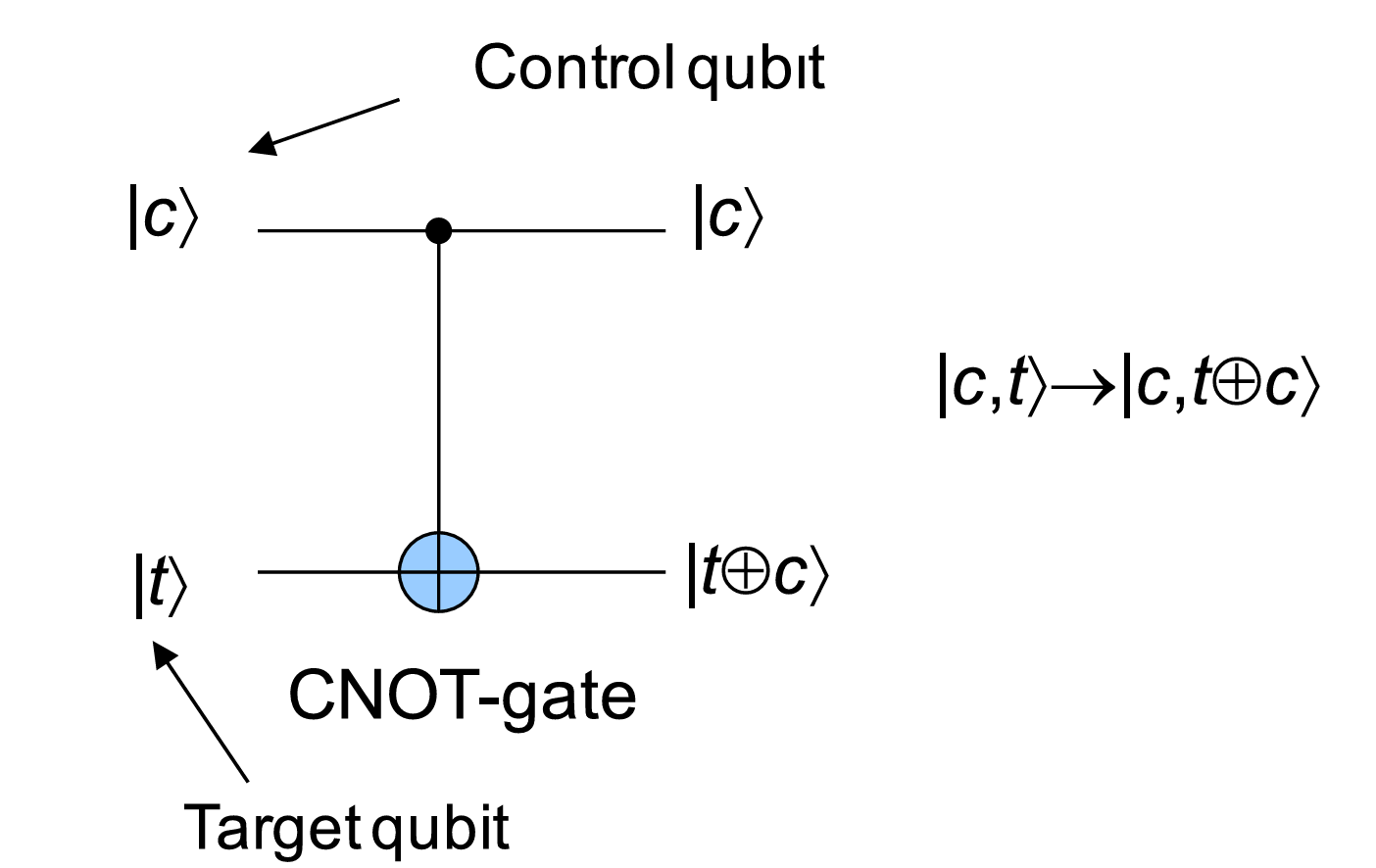
CNOT (controlled not) gate \(\begin{bmatrix}1 &&&\\& 1 &&\\&&0&1\\&&1&0\end{bmatrix}:\begin{cases}\ket{00}\to\ket{00}\\\ket{01}\to\ket{01}\\\ket{10}\to\ket{11}\\\ket{11}\to\ket{10}\end{cases}\)

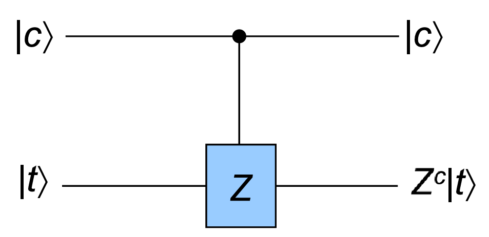
CPF (controlled phase flip) gate \(\begin{bmatrix}1 &&&\\& 1 &&\\&&1&\\&&&-1\end{bmatrix}:\begin{cases}\ket{00}\to\ket{00}\\\ket{01}\to\ket{01}\\\ket{10}\to\ket{10}\\\ket{11}\to-\ket{11}\end{cases}\)

Prop.

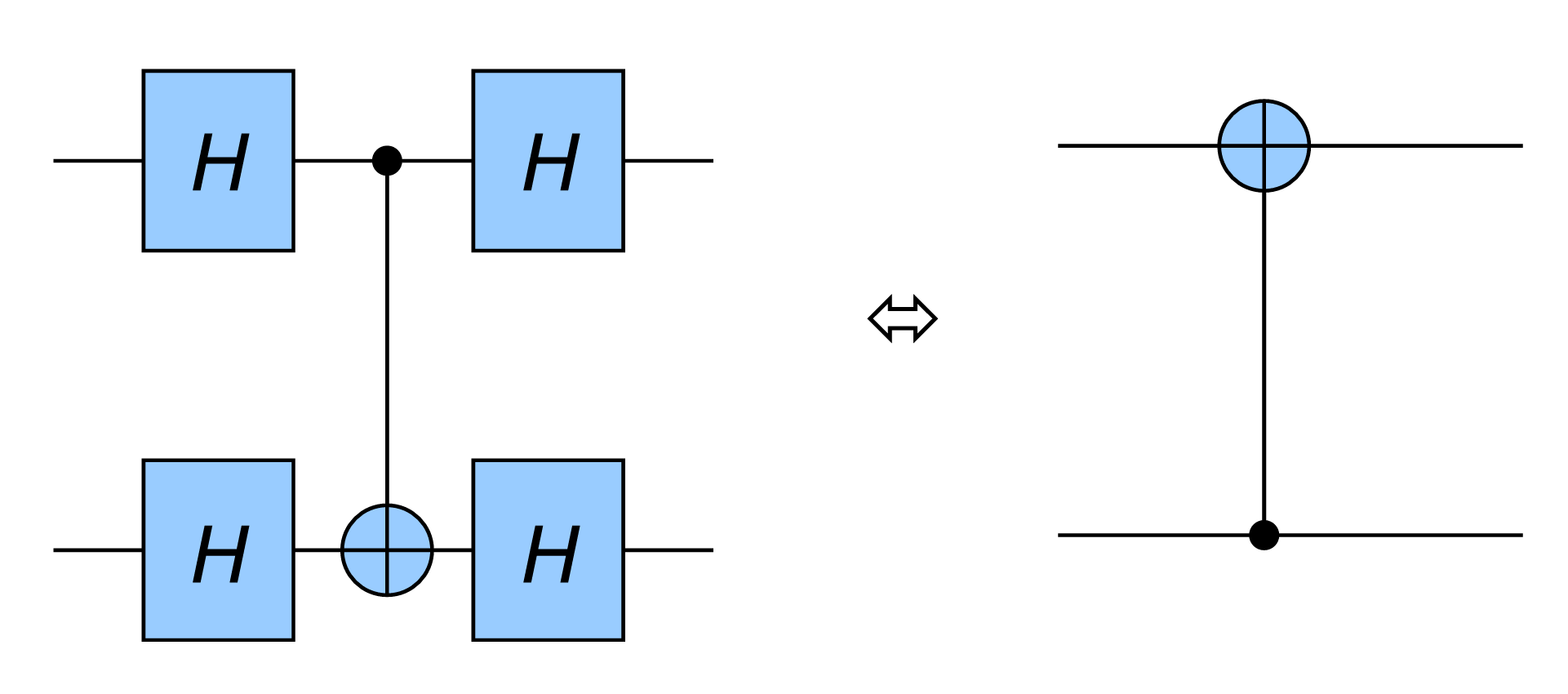
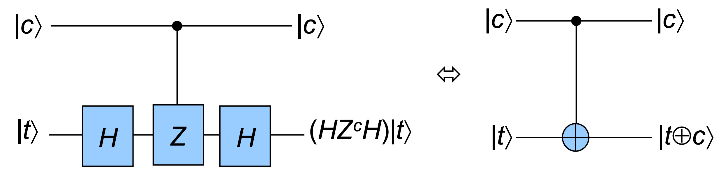
Basis change: \(Z\leftrightarrow X\) basis, control \(\leftrightarrow\) target.

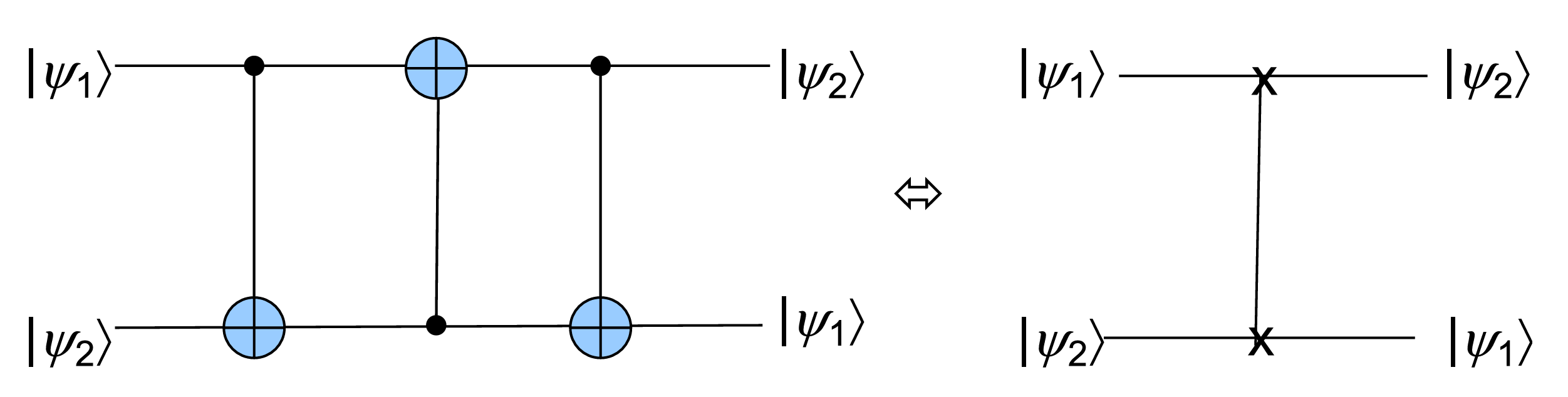
\(C_{12}C_{21}C_{12}=SWAP.\)

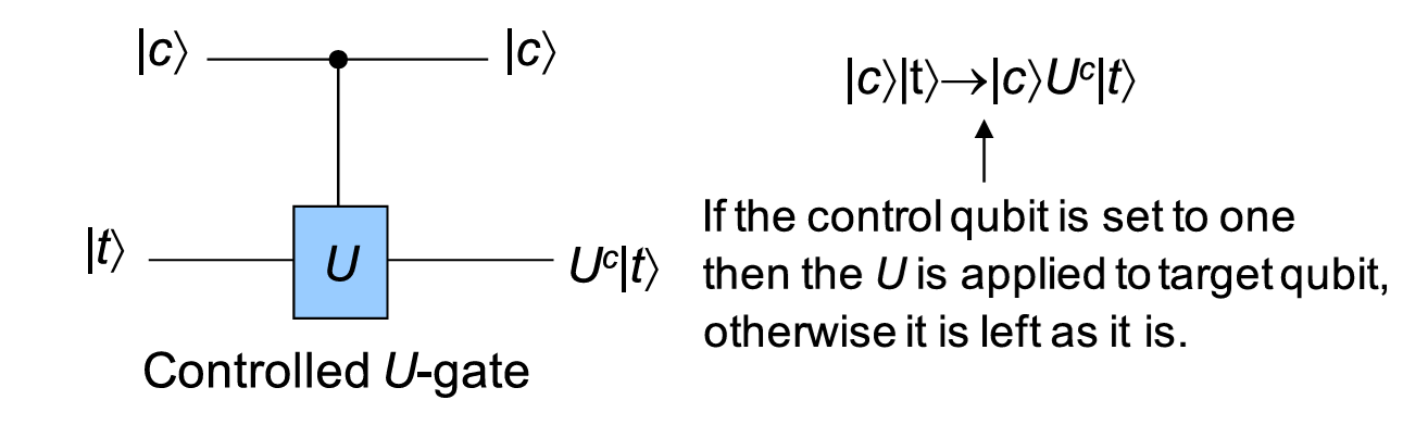
In general, \(C-U\) (controlled-\(U\)) gate \(\begin{bmatrix}I&\\&U\end{bmatrix}\)

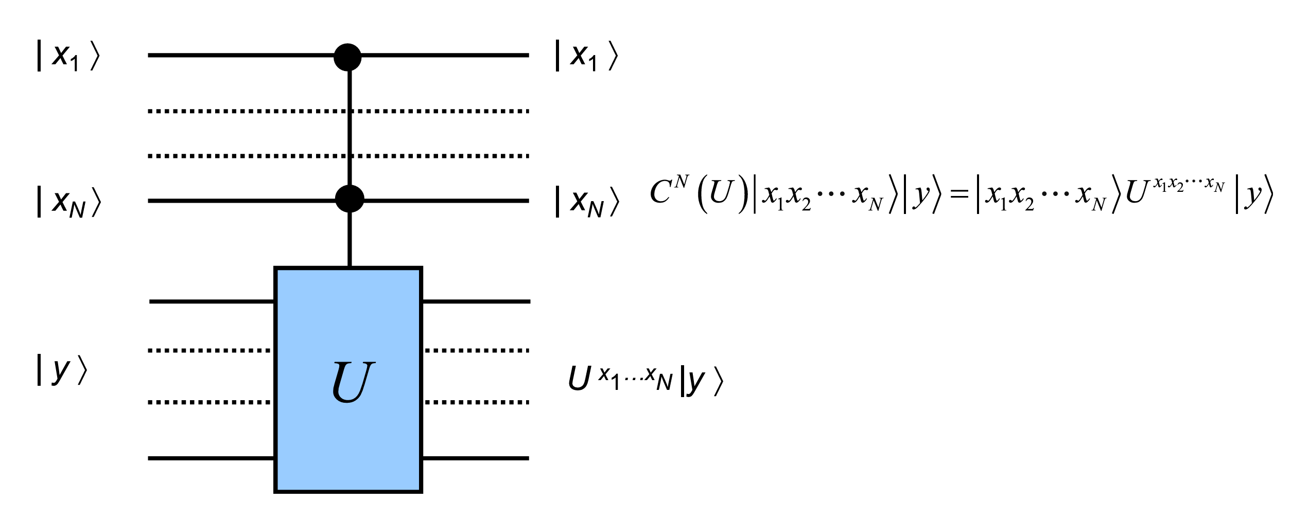
\(C^N-U\) gate:

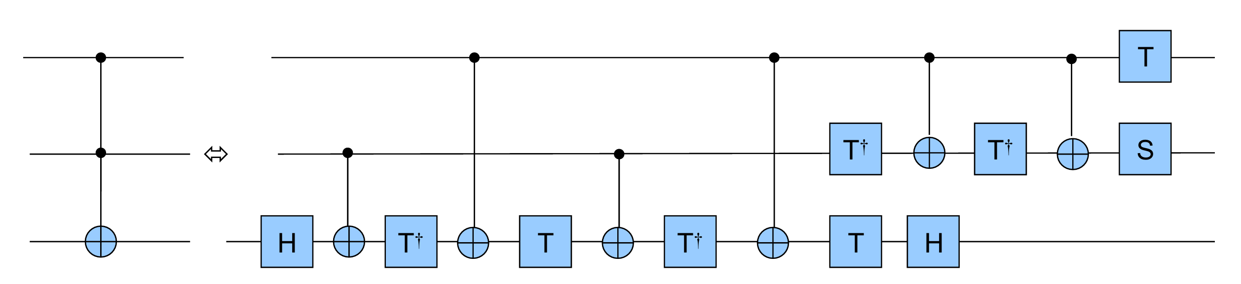
Toffoli gate \(C^2-X\):

Universality Theorem

Def. A Hamiltonian \(A\) is a generic operator if all the eigenvalues \(\theta_i\) of the \(A\) are irrational multiples of \(\pi\) and all the \(\theta_i\)'s are incommensurate (each \(\theta_i/\theta_j\) is also irrational).

Lem. \(e^A=\lim\limits_{n\to\infty}\left(1+\frac{A}{n}\right)^n.\)

Lem. If gates \(U=e^{iA}\) and \(U'=e^{iB}\) are realizable, where \(A,B\) are generic operators, we can realize any gate of the form

\[e^{i(\alpha A+\beta B)+\gamma[A,B]} \]

by a combination of \(U,U'\).

Pf. Idea: Irrational numbers are dense in the entire space. Let the eigenvalues of \(U\) be \(e^{i\theta_1},...,e^{i\theta_n}\). All \(\theta_i\) are irrational multiples of \(\pi\). Then \(U^n\) has eigenvalues \(e^{in\theta_i}(i=1,2,...,n)\). It can arbitrary approximates any real number.

Notice that we have

\[\lim\limits_{n\to\infty}\left(e^\frac{i\alpha A}{n}e^\frac{i\beta B}{n}\right)^n=\lim\limits_{n\to\infty}\left(1 +\frac{i}{n}(\alpha A+\beta B)\right)^n=e^{i(\alpha A+\beta B)}. \]

and

\[\lim\limits_{n\to\infty}\left(e^\frac{iA}{\sqrt{n}}e^\frac{iB}{\sqrt{n}}e^\frac{-iA}{\sqrt{n}}e^\frac{-iB}{\sqrt{n}}\right)^n=\lim\limits_{n\to\infty}\left(1 -\frac{1}{n}(AB-BA)\right)^n=e^{-[A,B]}. \]

by expanding to \(2^{nd}\) order.

Thm (Universality 1). CNOT + generic single-bit gates are universal.

Pf. Let \(U\) be a generic single-bit gate. \(U^n\) realize any single-bit gate. Let \(U_k\) be any single-bit gate

\(U_1C_{12}U_2\) realize generic 2-bit gate. \(U_1C_{12}U_2C_{13}U_3...\) realize generic \(n\)-bit gate.

Rem. CNOT can be replaced by CZ, but not SWAP.

Thm (Universality 2). Gates {CNOT, H, S(phase), T(gate)} are universal.

Pf. \(H,S,T\) are not generic, but

\[THTH=e^{-\frac{i\pi}{8}Z}e^{-\frac{i\pi}{8}X}=\cos^2\frac{\pi}{8}I-i\left(\cos\frac{\pi}{8}X+\sin\frac{\pi}{8}Y+\cos\frac{\pi}{8}Z\right)\sin\frac{\pi}{8} \]

Recall that a rotation along axis \(\vec{n}\) with rotation angle \(\theta\) is:

\[R_{\vec{n}}(\theta)=\exp\left(-i\frac{\theta}{2}\vec{n}\cdot\vec{\sigma}\right)=\cos\frac{\theta}{2}I-i\sin\frac{\theta}{2}(\vec{n}\cdot\vec{\sigma}). \]

so \(THTH\) is a rotation along axis \(\vec{n}=(\cos\frac{\pi}{8},\sin\frac{\pi}{8},\cos\frac{\pi}{8})\) with rotation angle \(\cos\frac{\theta}{2}=\cos^2\frac{\pi}{8}.\) We can show that it's generic.

Gate Simulation: Efficiency and Quantum Computation Complexity

Thm (Solovay-kitaer Theorem). For simulation of any single bit gate with a distance \(\epsilon\) from a discrete set, the number of steps needed is

\[O\left(\log^c\left(\frac{1}{\epsilon}\right)\right) \]

for some constant \(c\approx 2\).

In general, simulator of arbitrary \(U(2^n\times 2^n)\) with universal set of gates are inefficient (exponential growth in \(n\)). But simulation of constant \(m\)-bit state (some special \(N\)-bit gate \(C^N − U\)) are efficient.

Quantum Computation Complexity:

\[\mathsf{BQP}=\{\text{decision problem that can be solved with poly size quantum circuit with bounded error probability} \}.\\ \mathsf{BPP}=\{\text{decision problem that can be solved with poly size classical circuit with bounded error probability} \}.\\ \]

We have:

\[\mathsf{P\subseteq BPP\subseteq BQP\subseteq PSPACE} \]

OPEN PROBLEM: \(\mathsf{P}\overset{?}{=}\mathsf{PSPACE}\).

Other models of quantum computer

• Quantum Turning Machine
• Cluster (graph) state model
• Measurement model

Quantum Algorithms 1: Deutsch-Jozsa Algorithm, Grover search algorithm

Types of speed-up:

• non-exponential speedup: Grover search
• likely-exponential speedup: factorization, quantum simulation

Deutsch-Jozsa Algorithm

Deutsch's problem. Given a black box function \(f:\{0,1\}\to\{0,1\}\), determine whether \(f(0)=f(1)\).

If we are only allowed to give classical inputs, two visits are needed. But for quantum, one visit is enough!

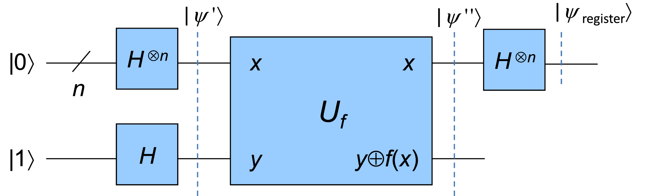
Alg (Deutsch Algorithm). Now we are presented with a quantum black box \(U_f\) that computes \(f:\{0,1\}\to\{0,1\}\):

\[U_f:\ket{x}\ket{y}\to\ket{x}\ket{y\oplus f(x)}. \]

Consider the following quantum circuit:

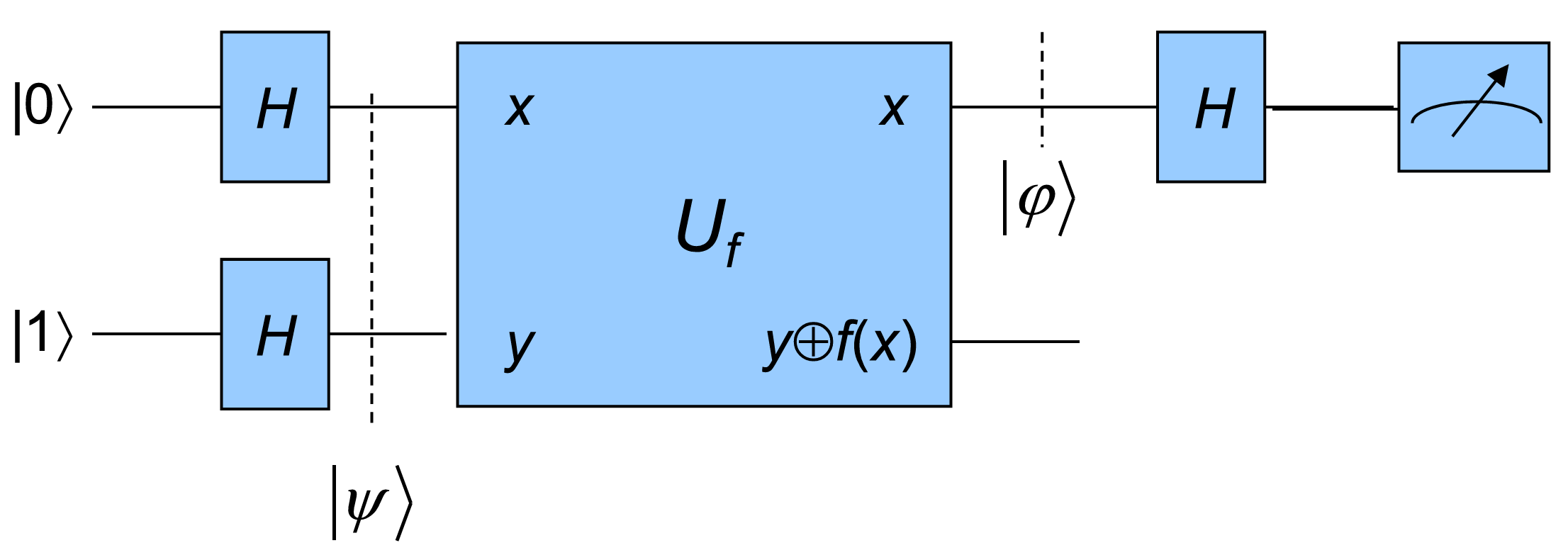
We can see that

\[\ket{\psi}=H\ket{0}\otimes H\ket{1}=\frac{1}{2}(\ket{0}+\ket{1})(\ket{0}-\ket{1})=\frac{1}{2}\left(\sum\limits_{x=0}^1\ket{x}\right)(\ket{0}-\ket{1}) \]

and

\[U_f\ket{\psi}=\frac{1}{2}U_f\left(\sum\limits_{x=0}^1\ket{x}\right)(\ket{0}-\ket{1})=\frac{1}{2}\left(\sum\limits_{x=0}^1(-1)^{f(x)}\ket{x}\right)(\ket{0}-\ket{1}). \]

Then

\[\ket{\varphi}=\frac{1}{\sqrt{2}}\left(\sum\limits_{x=0}^1(-1)^{f(x)}\ket{x}\right)=\frac{1}{\sqrt{2}}\left((-1)^{f(0)}\ket{0}+(-1)^{f(1)}\ket{1}\right). \]

Therefore,

\[\begin{align*} &\ H\ket{\varphi}\\ =&\ \frac{1}{2}\left((-1)^{f(0)}(\ket{0}+\ket{1})+(-1)^{f(1)}(\ket{0}-\ket{1})\right)\\ =&\ \frac{1}{2}\left((-1)^{f(0)}+(-1)^{f(1)}\right)\ket{0}+\frac{1}{2}\left((-1)^{f(0)}-(-1)^{f(1)}\right)\ket{1}\\ =&\ \begin{cases}\ket{0} & f(0)=f(1)\\\ket{1} & f(0)\neq f(1)\end{cases}. \end{align*} \]

Extension. The Deutsche-Jozsa algorithm represents a generalization of Deutsch’s algorithm. Namely, it verifies if the mapping \(f:\{0,1\}^n\to\{0,1\}\) is constant (\(f(x)=f(0)\) for all \(x\)) or balanced (\(f(x)=0\) for half \(x\)).

\[\ket{\psi'}=\frac{1}{2^{n/2}}\sum\limits_{x=0}^{2^n-1}\ket{x}(\ket{0}-\ket{1}),\\ \ket{\psi''}=U_f\ket{\psi'}=\frac{1}{2^{n/2}}\sum\limits_{x=0}^{2^n-1}(-1)^{f(x)}\ket{x}(\ket{0}-\ket{1}),\\ \ket{\psi_{\text{register}}}=H^{\otimes n}\frac{1}{2^{n/2}}\sum\limits_{x=0}^{2^n-1}(-1)^{f(x)}\ket{x}=\frac{1}{2^{n}}\sum\limits_{x=0}^{2^n-1}\sum\limits_{y=0}^{2^n-1}(-1)^{f(x)}(-1)^{xy}\ket{y}. \]

Now we consider

\[c_y=\braket{y|\psi_{\text{register}}}=\frac{1}{2^{n}}\sum\limits_{x=0}^{2^n-1}(-1)^{f(x)}(-1)^{xy}. \]

• If \(f\) is constant:

  \[c_y=\frac{(-1)^{f(0)}}{2^n}\sum\limits_{x=0}^{2^n-1}(-1)^{xy}=(-1)^{f(x)}\delta_{y,0} \]

• If \(f\) is balanced:

  \[c_0=\frac{1}{2^n}\sum\limits_{x=0}^{2^n-1}(-1)^{f(x)}=0. \]

Therefore, checking whether the measurement is \(\ket{0}\) can distinguish between these two cases.

Grover search algorithm

Problem. Given an unstructured data base with \(N\) entries, search for a specific entry.

A classical algorithm will take on average \(\frac{N}{2}\) attempts, while the Grover search algorithm solves this problem in \(\sim \sqrt{N}\) operations.

Alg (Grover search). Assume \(N=2^n\), the data base address contains \(n\) qubits and the search function is defined by \(f_w:\{0,1\}^{\otimes n}\to\{0,1\}\):

\[f_w(x)=\begin{cases}0 & x\neq w\\1 & x=w\end{cases}. \]

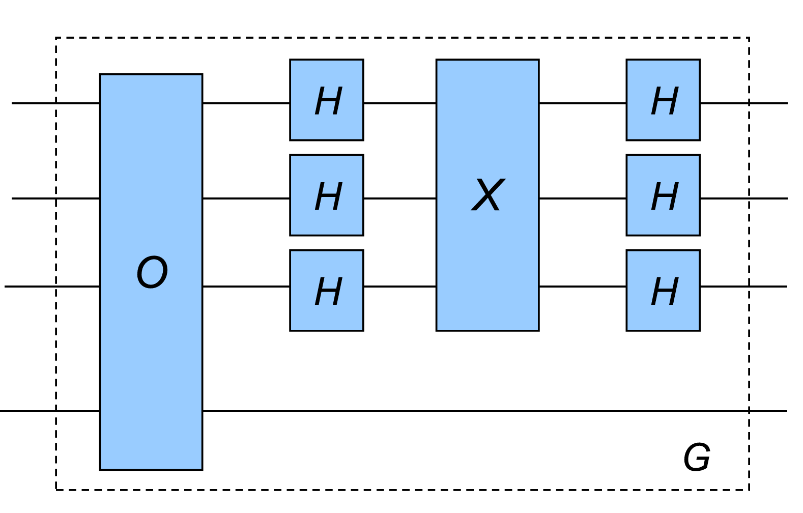
meaning that the search function result is one if the correct item \(\ket{w}\) is found. The corresponding quantum box is

\[U_w:\ket{x}\ket{y}\to\ket{x}\ket{y\oplus f_w(x)}. \]

Since \(U_w\ket{x}(\ket{0}-\ket{1})=(-1)^{f_w(x)}\ket{x}(\ket{0}-\ket{1})\), we have the oracle operator

\[O_w:\ket{x}\to(-1)^{f_w(x)}\ket{x}=(I-2\ket{w}\bra{w})\ket{x}. \]

Based on it, we define the Grover operator by:

\[G=H^{\otimes n}XH^{\otimes n}O_w \]

where \(X\ket{x}=-(-1)^{\delta_{x0}}\ket{x}\) or \(X=2\ket{0}\bra{0}-I\). Let

\[\ket{\Psi}=H^{\otimes n}\ket{0^{\otimes n}}=\frac{1}{2^{n/2}}\sum\limits_{i=0}^{2^n-1}\ket{x}. \]

Then

\[G=H^{\otimes n}(2\ket{0}\bra{0}-I)H^{\otimes n}O_w=\left(2\ket{\Psi}\bra{\Psi}-I\right)O_w. \]

We can write

\[\ket{\Psi}=\frac{1}{2^{n/2}}\sum\limits_{i=0}^{2^n-1}\ket{x}=\sqrt{1-\frac{1}{N}}\ket{\alpha}+\sqrt{\frac{1}{N}}\ket{w} \]

where

\[\ket{\alpha}=\sqrt{\frac{1}{N-1}}\sum\limits_{x\neq w}\ket{x}. \]

By substituting \(\sqrt{1-\frac{1}{N}}=\cos\left(\frac{\theta}{2}\right)\) gives

\[\ket{\Psi}=\cos\left(\frac{\theta}{2}\right)\ket{\alpha}+\sin\left(\frac{\theta}{2}\right)\ket{w}. \]

Let's now apply the oracle operator on \(\lambda\ket{\alpha}+\mu\ket{w}\) to obtain:

\[O_w(\lambda\ket{\alpha}+\mu\ket{w})=\lambda\ket{\alpha}-\mu\ket{w}. \]

The Grover operator action on state \(\lambda\ket{\Psi}+\mu\ket{\Phi}\) is given by:

\[(2\ket{\Psi}\bra{\Psi}-I)(\lambda\ket{\Psi}+\mu\ket{\Phi})=\lambda\ket{\Psi}-\mu\ket{\Phi}. \]

Thus

\[G\ket{\Psi}=\cos\left(\frac{3\theta}{2}\right)\ket{\alpha}+\sin\left(\frac{3\theta}{2}\right)\ket{w}. \]

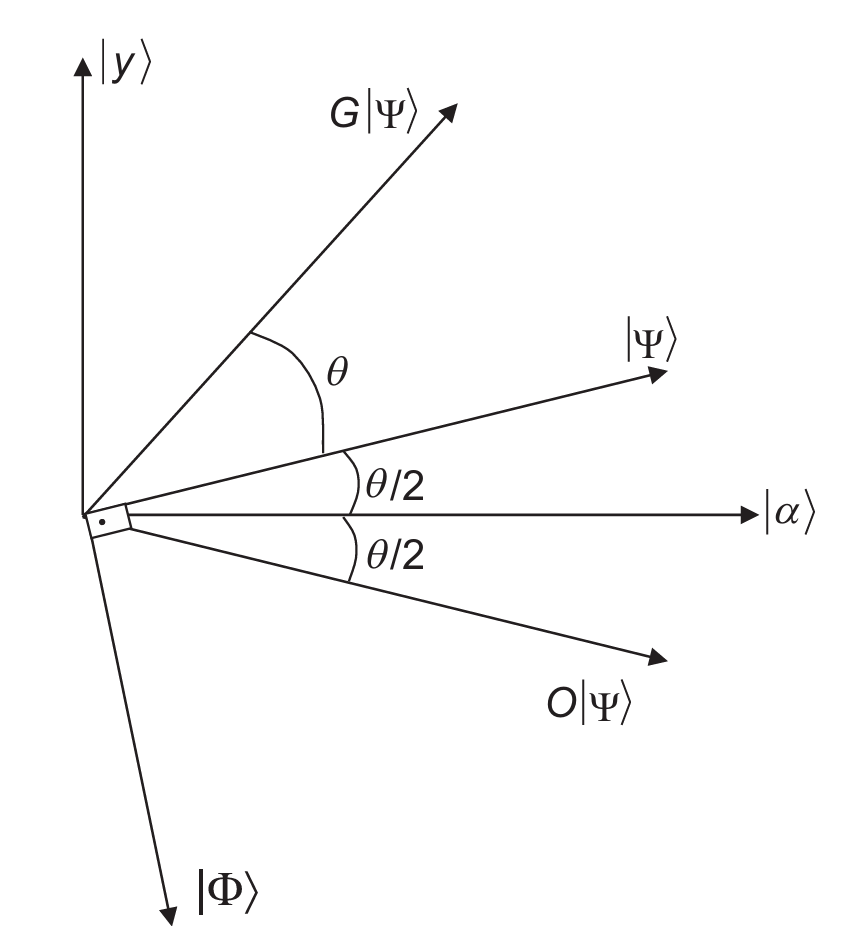
Similarly,

\[G^k\ket{\Psi}=\cos\left(\frac{(2k+1)\theta}{2}\right)\ket{\alpha}+\sin\left(\frac{(2k+1)\theta}{2}\right)\ket{w}. \]

We want to find \(\ket{w}\), in other words,

\[\cos\left(\frac{(2k+1)\theta}{2}\right)=0. \]

Substituting \(\cos\left(\frac{\theta}{2}\right)=\sqrt{1-\frac{1}{N}}\) gives

\[k\sim\frac{\pi}{4}\sqrt{N}. \]

Thm. Grover algorithm is optimal: by any quantum circuit, visit \(T\ge \frac{\pi}{4}\sqrt{N}(1-\epsilon)(\epsilon\to 0 \text{ or }N\to\infty)\).

Quantum Algorithms 2: Quantum Simulation, Quantum Fourier Transform and Shor's factorization algorithm.

Quantum Simulation

Quantum simulation is the idea of using one quantum mechanical system to simulate another quantum mechanical system more efficiently than can be achieved by any system based on classical physics.

Def. \(k\)-local Hamiltonian is like

\[H=\sum_ix_{i\mu}\sigma_{i\mu}+\sum_{ij}x_{ij\mu\nu}\sigma_{i\mu}\sigma_{j\nu}+\ldots+\sum\limits_{i_1i_2...i_k}x_{i_1...i_k\mu_1...\mu_k}\sigma_{i_1\mu_1}...\sigma_{i_k\mu_k} \]

Prob. Input: Constant-local Hamiltonian \(H=\sum_k H_k\), initial state \(\ket{\psi(0)}\), accuracy \(\delta\), time \(t_f\).

Output: State \(\ket{\tilde{\psi}(t_f)}\) s.t. \(\left|\braket{\tilde{\psi}(t_f)|e^{-iHt_f}|\psi(0)}\right|^2\ge 1-\delta.\)

Thm. Let \(A\) and \(B\) be Hamiltonians. For any real \(t\),

\[\lim\limits_{n\to \infty}\left(e^{iAt/n}e^{iBt/n}\right)^n=e^{i(A+B)t} \]

even if \([A,B]\neq 0\).

Pf.

\[\left(e^{iAt/n}e^{iBt/n}\right)^n=I+\sum\limits_{k=1}^n\binom{n}{k}\frac{1}{n^k}[i(A+B)t]^k+O\left(\frac{1}{n}\right). \]

and \(\binom{n}{k}\frac{1}{n^k}=(1+O(\frac{1}{n}))/k!\).

Prop.

\[e^{i(A+B)\Delta t}=e^{iA\Delta t}e^{iB\Delta t}+O(\Delta t^2),\\ e^{i(A+B)\Delta t}=e^{iA\Delta t/2}e^{iB\Delta t}e^{iA\Delta t/2}+O(\Delta t^3).\\ \]

Alg. Pick \(\Delta t=\text{poly}(\delta)t_f\). Repeatedly do \(\ket{\psi}\gets U_{\Delta t}\ket{\psi}\), where \(U_{\Delta t}\) is an efficient circuit to simulate \(e^{-iH\Delta t}\).

Quantum Fourier Transform

Def. The unitary FT \(U_{\text{FT}}\):

\[\braket{y|U_{\text{FT}}|x}=\frac{1}{2^{n/2}}e^{2\pi ixy/2^n}. \]

Let \(\ket{\Psi}\) be a linear superposition of vector \(\ket{x}\):

\[\ket{\Psi}=\sum\limits_{x=0}^{2^n-1}f(x)\ket{x}, \]

where \(f(x)=\braket{x|\Psi}\). By applying \(U_{\text{FT}}\) we obtain

\[\ket{\Phi}=U_{\text{FT}}\ket{\Psi}=\sum\limits_{x=0}^{2^n-1}f(x)U_{\text{FT}}\ket{x}. \]

So the probability amplitude of finding the state \(\ket{y}\) is

\[\braket{y|\Phi}=\sum\limits_{x=0}^{2^n-1}f(x)\bra{y}U_{\text{FT}}\ket{x}=\frac{1}{2^{n/2}}\sum\limits_{x=0}^{2^n-1}f(x)e^{2\pi ixy/2^n}. \]

which is just the FT of \(f(x)\). The action of \(U_{\text{FT}}\) on \(\ket{x}\) in operator notation is given by:

\[\begin{align*} &\ U_{\text{FT}}\ket{x}\\ =&\ \frac{1}{2^{n/2}}\sum\limits_{y=0}^{2^n-1}e^{2\pi ixy/2^n}\ket{y}\\ =&\ \frac{1}{2^{n/2}}\sum\limits_{y=0}^{2^n-1}\prod\limits_{k=0}^{n-1}e^{2\pi ixy_k/2^{n-k}}\ket{y}\\ =&\ \frac{1}{2^{n/2}}\bigotimes_{k=0}^{n-1}\left(\ket{0}+e^{2\pi ix/2^{n-k}}\ket{1}\right)\\ \end{align*} \]

Define

\[R_d\equiv\begin{bmatrix}1 & 0\\0 & e^{i\pi/2^d}\end{bmatrix} \]

Let \(C_{ij}(R_d)\) denote the control-\(R_d\) gate, where \(i\) is the control qubit and \(j\) is the target qubit.

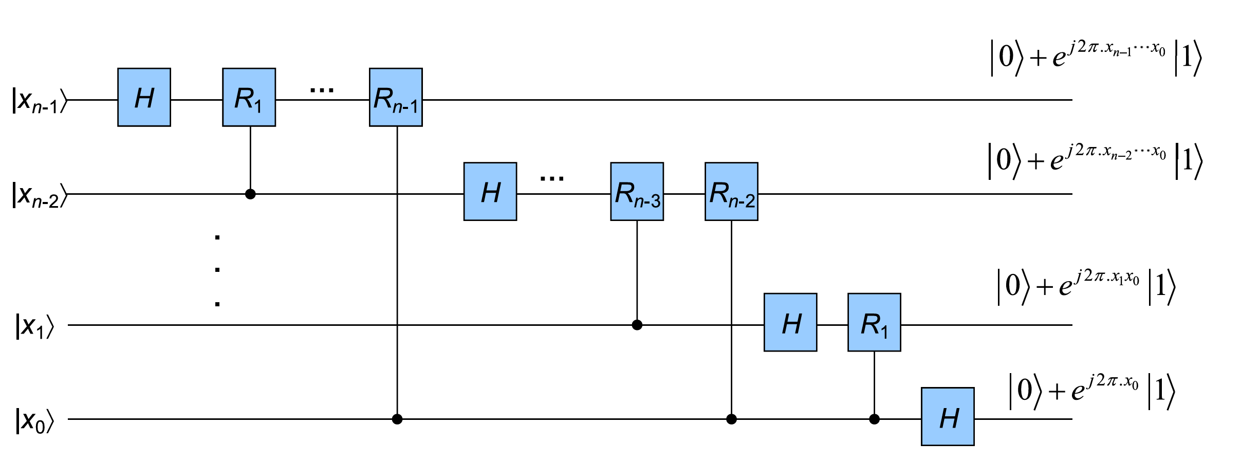
Cost: \(n\) \(H\)-gate and \(\frac{n(n-1)}{2}\) control-\(R_d\) gate. Therefore the overall complexity of the FT computation circuit is \(O(n^2)\).

Period Finding

Given \(f:\{0,1,...,N-1\}\to\{0,1\}^m\) satisfying \(f(x)=f(x+r)\) for some unknown \(r\), find it.

The initial state of \(n+m\) qubits is given by:

\[\ket{\Phi}=\frac{1}{\sqrt{N}}\left(\sum_{x=0}^{N-1}\ket{x}\right)\otimes\ket{0\cdots0}. \]

By applying the function operator, we obtain

\[\ket{\Phi_f}=U_f\ket{\Phi}=\frac{1}{\sqrt{N}}\sum_{x=0}^{N-1}\ket{x,f(x)}. \]

We now perform the measurement of the output register and obtain the result \(f_0\), the corresponding final state of the first register will be “the state vector collapse”:

\[\ket{\Psi}=\frac{1}{\sqrt{K}}\sum\limits_{f(x)=f_0}\ket{x}=\frac{1}{\sqrt{K}}\sum\limits_{k=0}^{K-1}\ket{x_0+kr} \]

where \(x_0\) is the minimum \(x\) to satisfy \(f(x_0)=f_0\). Clearly,

\[K=\left\lfloor\frac{N}{r}\right\rfloor\text{ or }\left\lfloor\frac{N}{r}\right\rfloor+1. \]

Then perform QFT on it:

\[\ket{\Psi'}=U_{\text{FT}}\ket{\Psi}=\frac{1}{\sqrt{NK}}\sum_{y=0}^{N-1}e^{2\pi ix_0y/N}\sum_{k=0}^{K-1}e^{2\pi i(kr)y/N}\ket{y} \]

Measuring it in computational basis \(\{y\}\) gives

\[\text{prob}(y)=\frac{1}{NK}\left| \sum_{k=0}^{K-1}e^{2\pi i(kr)y/N}\right|^2 \]

which is strongly peaked where $\dfrac{ry}{N}\sim $ integer.

By analysis, when \(\frac{kN}{r}-\frac{1}{2}\le y\le \frac{kN}{r}+\frac{1}{2}\),

\[\text{prob}(y)\ge \frac{4}{\pi}\frac{1}{r}. \]

Thus one finds \(\frac{k}{r}\) where \(k\) is randomly sampled in \(\{0,1,...,r-1\}\) with probability \(\ge\frac{4}{\pi}\).

If \(k,r\) are relatively prime, immediately find \(r\). Such case has constant probability.

Factoring

Alg (Shor's factorization algorithm). Given an integer \(N\):

1. Randomly generate an integer \(a\) between \(0\) and \(N-1\), determine the \(\gcd(a,N)\). If \(\gcd(a,N) > 1\), then \(a\) is a nontrivial factor of \(N\); otherwise go to next step.
2. Consider function \(f(x)\equiv a^x\bmod N\), use the above algorithm to find the period of \(f(x)\).
3. Suppose period is \(r\), so \(a^r\equiv 1\pmod N\). If \(N\) is factorizable, with prob \(\sim \frac{1}{2}\), \(r\) is even. Compute \(\gcd(a^{r/2}-1,N)=p\) and \(\gcd(a^{r/2}+1,N)=q\) to check if either \(p\) or \(q\) is a nontrivial factor.

Quantum Error Correction

The initial state \(\rho\) passes through the quantum channel with noise to obtain

\[\hat{\mathcal{E}}(\rho)=\sum_iE_i\rho E_i^\dagger \]

where \(\{E_i\}\) are the error operators satisfying \(\sum_iE_iE_i^\dagger=I\).

Condition for Q.E.C

Thm. Let \(C\) be a quantum code, \(P\) be a projector onto \(C\). The errors \(\{E_i\}\) are correctable, i.e., \(\exists \hat{R}\) s.t. \(P\hat{R}\hat{\mathcal{E}} P=P\hat{I}P\) if and only if \(PE_i^\dagger E_jP=\alpha_{i,j}P\) for some \(\alpha_{i,j}\in \mathbb{C}\).

Rem.

• \(\alpha_{ij}\propto \delta_{ij}\): Non-degenerate Code. Different errors are orthogonal in the code space and can be uniquely identified and corrected.
• \(\alpha_{ij}=c\): Decoherence-Free Subspace. The errors are indistinguishable, but the code space is immune to noise (no active error correction is required).

Thm. If errors \(\{E_i\}\) are correctable, any superposition \(\{F_j=\sum_i\rho_{ji}E_i\}\) are also correctable.

Pf.

\[PF_j^\dagger F_{j'}P=\sum_{ii'}\rho_{ji}\rho_{j'i'}PE_i^\dagger E_{i'}P=\sum_{ii'}\rho_{ji}\rho_{j'i'}\alpha_{ii'}P. \]

Rem. Only need to consider a discrete set of errors.

Thm (Quantum Hamming bound). Non-degenerately encode \(k\) bits information to \(n\) quantum bits so that arbitrary \(\le t\)-bit error can be corrected, then

\[\sum\limits_{j=0}^t\binom{n}{j}3^j2^k\le 2^n. \]

Pf. The number of errors is

\[\sum\limits_{j=0}^t\binom{n}{j}3^j. \]

each error corresponds to a \(k\)-dim subspace, so

\[\sum\limits_{j=0}^t\binom{n}{j}3^j2^k\le 2^n. \]

Cor. For \(k=t=1\), \(n\ge 5\).

Stabilizer Codes

Let \(g_1,g_2...,g_{n-k}\) be independent and pairwise commutative stabilizers in \(n\)-bit system. \(S\) is the \(k\)-dim subspace generated by them. Pick \(\bar{Z}_1,...,\bar{Z}_k\) so that \(g_1,...,g_{n-k},\bar{Z}_1,...,\bar{Z}_k\) are independent and pairwise commutative. Encode \(\ket{x_1...x_k}_L\) to the stable state of \(g_1,...,g_{n-k},(-1)^{x_1}\bar{Z_1},...,(-1)^{x_k}\bar{Z}_k\).

Similarly, define \(\bar{X}_j\) s.t. \(\bar{X}_j\bar{Z}_j=-\bar{Z}_j\). So \(\bar{X}_j\) is like "not" gate for logic state. To correct error, measure stabilizer \(\{g_i\}\) to get syndrome (\(\pm 1\)), then recovery.

Ex. \(n=5,t=1,k=1\).

Operator	Content
\(g_1\)	\(XZZXI\)
\(g_2\)	\(IXZZX\)
\(g_3\)	\(XIXZZ\)
\(g_4\)	\(ZXIXZ\)
\(\bar{Z}\)	\(ZZZZZ\)
\(\bar{X}\)	\(XXXXX\)

One can verify that

\[\begin{cases} \bar{Z}\ket{0}_L=\ket{0}_L\\ \bar{Z}\ket{1}_L=-\ket{1}_L\\ \bar{X}\ket{0}_L=\ket{1}_L\\ \bar{X}\ket{1}_L=\ket{0}_L \end{cases}. \]

Fault-tolerant Quantum Computation

All the elements (state preparation, gates, measurement) have a constant and independent error rate \(p\).

Replace single qubit with a block. Implement each element fault-tolerantly: one-element fail will only lead to a one-bit error in each block. Since one-bit error is correctable, have error after correction with probability \(cp^2\), for some constant \(c\).

Concatenation: Encode \(C_0\) to \(C_1\), \(C_1\) to \(C_2\), ..., \(C_{k-1}\) to \(C_k\). Error probability is

\[p_f^{(2)}=cp^2,p_f^{(3)}=c(cp^2)^2=c^3p^4,p_f^{(k)}=\frac{(cp)^{2^k}}{c} \]

can be arbitrarily small if \(p<\frac{1}{c}=p_{\text{th}}\).

If we need \(n\)-gates for a computation, each gate is \(k\)-level concatenation, the error of while computation

\[p_f^{(k)}\cdot n\le \varepsilon. \]

Substituting gives

\[2^k\ge\log\left(\frac{c\varepsilon}{n}\right)/\log (cp). \]

For each concatenation, one gate is replaced with \(d\) gates (operations). After \(k\)-levels, total cost of one gate is

\[d^k=\left(\frac{\log\left(\frac{c\varepsilon}{n}\right)}{\log (cp)}\right)^{\log d}=O(\text{poly}(\log(n/\varepsilon))). \]

Thm (Error Threshold Theorem). If error per quantum operations is smaller than a constant threshold \(P_{\text{th}}\), the error of whole computation can be reduced to an arbitrary level \(\varepsilon\) with additional cost \(O(\text{poly}(\log(n/\varepsilon))).\)