Cryptography
Classical Cryptography
Private-key Encryption and Perfect Secrecy
First, we formally give some notations to demonstrate an encryption protocol.
Def (Private-key Encryption). The triplet of algorithms \((\mathsf{Gen, Enc, Dec})\) is called a private-key encryption scheme over the message space \(\mathcal{M}\) and the key space \(\mathcal{K}\) if the following holds:
- \(\mathsf{Gen}\) (called the key generation algorithm) is a randomized algorithm that returns a key \(k\) such that \(k \in \mathcal{K}\). We denote by \(k \leftarrow Gen\) the process of generating a key \(k\).
- \(\mathsf{Enc}\) (called the encryption algorithm) is a potentially randomized algorithm that on input a key \(k \in \mathcal{K}\) and a message \(m \in \mathcal{M}\), outputs a ciphertext \(c\). We denote by \(c \leftarrow \mathsf{Enc}_k(m)\) the output of Enc on input key \(k\) and message \(m\).
- \(\mathsf{Dec}\) (called the decryption algorithm) is a deterministic algorithm that on input a key \(k\) and a ciphertext \(c\) outputs a message \(m\).
- (Correctness) \(\forall m \in \mathcal{M}\),
Rem. Note that we only assume key \(k\) to be private in this scheme, other things such as the \(\mathsf{Gen, Enc, Dec}\) algorithms are exposed to adversaries.
To evaluate the secrecy for a private-key encryption scheme, we introduce provable secrecy, it mainly concludes Shannon's secrecy and Perfect secrecy. Later we'll show the equivalence of them.
Def (Shannon Secrecy). \((\mathcal{M}, \mathcal{K}, \mathsf{Gen}, \mathsf{Enc}, \mathsf{Dec})\) is said to be a private-key encryption scheme that is Shannon-secret with respect to the distribution \(D\) over the message space \(\mathcal{M}\) if for all \(m^{\prime} \in \mathcal{M}\) and for all \(c\),
An encryption scheme is said to be Shannon secret if it is Shannon secret with respect to all distributions \(D\) over \(\mathcal{M}\).
The intuition of this formula is that given the ciphertext \(c\), it could not reveal any new information to the message \(m\). In fact, the only thing that adversaries could learn is still the priori information.
Def (Perfect Secrecy). A tuple \((\mathcal{M}, \mathcal{K}, \mathsf{Gen}, \mathsf{Enc}, \mathsf{Dec})\) is said to be a private-key encryption scheme that is perfectly secret if for all \(m_1, m_2 \in \mathcal{M}\), and for all \(c\),
Now we'll show that in fact these two definitions are equivalent.
Thm. A scheme \((\mathcal{M}, \mathcal{K}, \mathsf{Gen}, \mathsf{Enc}, \mathsf{Dec})\) is Shannon's secrecy if and only if it's perfect secrecy.
Pf.
(1) Perfect secrecy \(\Rightarrow\) Shannon's secrecy:
Our goal is to prove that
First, according to the definition of conditional probability, the left-hand side could be rewritten as
Now we only need to prove that \(\text{Pr}_{k}\left[\mathsf{Enc}_k(m^{\prime})=c\right] = \text{Pr}_{k,m}\left[\mathsf{Enc}_k(m)=c\right]\).
Notice that
(2) Perfect secrecy \(\Leftarrow\) Shannon's secrecy:
Since Shannon's secrecy holds for all distributions \(D\), it holds for a specific distribution. We consider the special case where \(D\) only chooses between two given messages.
Consider \(m_1, m_2 \in \mathcal{M}\), and \(D\) is the uniform distribution over \({m_1, m_2}\) and any ciphertext \(c\). We show that
Note that the definition of \(D\) implies \(\text{Pr}_m[m=m_1] = \text{Pr}_m[m=m_2] = \frac{1}{2}\), therefore, follows by Shannon's secrecy
By the definition of conditional probability,
Analogously,
Canceling and rearranging terms, we conclude that
One-Time Pad
Def (One-Time Pad Encryption Scheme). The One-Time Pad encryption scheme is described by the following 5-tuple \((\mathcal{M}, \mathcal{K}, \mathsf{Gen}, \mathsf{Enc}, \mathsf{Dec})\):
The \(\oplus\) operator represents the binary xor operation.
Prop. The One-Time Pad is a perfectly secure private-key encryption scheme.
Pf. The proof is quite straightforward. Since the choice of \(k\) is arbitrarily from \(\{0,1\}^n\), it's obvious that
And
Thus, we can conclude that
Properties and Limitations of Perfect Secrecy
Thm (Shannon's Theorem). If scheme \((\mathcal{M}, \mathcal{K}, \mathsf{Gen}, \mathsf{Enc}, \mathsf{Dec})\) is a perfectly secret private-key encryption scheme, then \(|\mathcal{K}| \geq |\mathcal{M}|\).
Proof. We achieve the proof through contradiction. Assume there exists a perfectly secret private-key encryption scheme \((\mathcal{M}, \mathcal{K}, \mathsf{Gen}, \mathsf{Enc}, \mathsf{Dec})\) such that \(|\mathcal{K}| < |\mathcal{M}|\). Take any \(m_1 \in \mathcal{M}, k \in \mathcal{K}\), and let \(c \leftarrow \mathsf{Enc}_k(m_1)\). Let \(\mathsf{Dec}(c)\) denote the set \(\{m = \mathsf{Dec}_k(c) \mid \exists k \in \mathcal{K}\}\) of all possible decryptions of \(c\) under all possible keys. Since the algorithm \(\mathsf{Dec}\) is deterministic, this set has size at most \(|\mathcal{K}|\). But since \(|\mathcal{M}| > |\mathcal{K}|\), there exists some message \(m_2\) not in \(\mathsf{Dec}(c)\). By the definition of a private encryption scheme, it follows that
But since
we conclude that
Here is a theorem to help demonstrate Shannon's secrecy.
Thm. Let \((\mathsf{Gen}, \mathsf{Enc}, \mathsf{Dec})\) be an encryption scheme with message space \(\mathcal{M}\), for which \(|\mathcal{M}| = |\mathcal{K}| = |\mathcal{C}|\). The scheme is perfectly secret if and only if:
- Every key \(k \in \mathcal{K}\) is chosen with (equal) probability \(\frac{1}{|\mathcal{K}|}\).
- For every \(m \in \mathcal{M}\) and every \(c \in \mathcal{C}\), there exists a unique key \(k \in \mathcal{K}\) such that \(\mathsf{Enc}_k(m)\) outputs \(c\).
Proof. The intuition behind the proof of this theorem is as follows. To see that the statement implies perfect secrecy, the second condition implies the mapping from \(m \to c\) is one-to-one, and \(\mathcal{M} = \mathcal{C}\) implies it's one-to-one and onto. And then, combined with the first statement, we can conclude that \(\text{Pr}_k[\mathsf{Enc}_k(m)=c] = \frac{1}{|\mathcal{K}|}\).
To see the other direction, we consider a fixed \(c \in \mathcal{C}\) such that \(\text{Pr}_k[\mathsf{Enc}_k(m)=c] > 0\). For such \(c\), we could consider \(\mathsf{Enc}\) as a mapping from \(m\) to \(k\) because \(\text{Pr}[\mathsf{Enc}_k(m)=c] > 0\) is identical for every \(m\). This mapping is one-to-one for correctness. And similarly, since \(|\mathcal{M}| = |\mathcal{K}|\), it's one-to-one and onto. Hence, \(\forall m_1, m_2 \in \mathcal{M}\), we have
Hence, we finish the proof.
Computational Hardness
One-Way Functions
Def (Efficient algorithm). An algorithm is efficient if on inputs of length \(n\), its running time \(T(n)\) is polynomial in \(n\), meaning that there exists a constant \(c\) such that \(T(n)\leq n^c\).
Def (Non-uniform PPT). A non-uniform probabilistic polynomial-time machine (abbreviated n.u. p.p.t.) \(A\) is a sequence of probabilistic machines \(A = \{A_1, A_2,...\}\) for which there exists a polynomial \(d\) such that the description size of \(A_i < d(i)\) and the running time of \(A_i\) is also less than \(d(i)\). We write \(A(x)\) to denote the distribution obtained by running \(A_{|x|}(x)\).
Remark. For the simplicity of definition and modeling, we assume the adversary is non-uniform. When we use the word "p.p.t." for adversaries below, we mean n.u.p.p.t. instead.
Def (Negligible function). A function \(\varepsilon(n)\) is negligible if for every \(c\), there exists some \(n_0\) such that for all \(n>n_0\), \(\varepsilon(n)\leq 1/n^c\).
Intuitively, we want functions that are efficient to compute, but hard to invert. Here, to invert the function means to find any input \(x\) in the preimage of a given output \(y\). To capture this intuition, we have the following definitions for one-way functions.
Def (Worst-case one-way function). A function \(f:\{0,1\}^*\rightarrow\{0,1\}^*\) is worst-case one-way if
-
There is a p.p.t. \(M\) which computes \(f\), and
-
There is no p.p.t. \(A\) such that \(\exists n_0>0,\forall n>n_0,\forall x\in\{0,1\}^n\), we have
\[\Pr[x'\leftarrow A(1^n, f(x)):f(x')=f(x)]=1. \]
Rem. Although \(M\) by definition can be a randomized algorithm, in real world applications, it is usually deterministic, since \(f\) should be deterministic.
Rem. The existence of worst-case one-way functions is equivalent to \(\mathsf{NP\not\subseteq BPP}\).
Rem. The reason why we need \(1^n\) to be part of \(A\)'s input is that \(x\) could be much longer than \(y\), so that simply outputting \(x\) could take super-polynomial time. Adding \(1^n\) avoids this problem.
However, we do not know how to build a useful encryption scheme from worst-case one-way functions. In this sense, we need another definition for one-way functions.
Def (Strong one-way function). A function \(f:\{0,1\}^*\rightarrow\{0,1\}^*\) is strong one-way (or equivalently, one-way) if
- There is a p.p.t. \(M\) which computes \(f\), and
- For any p.p.t. \(A\) there is a negligible function \(\varepsilon(n)\) such that
Remark. Note that the distribution of \(x\) is uniform over \(\{0,1\}^n\) if not specified. There is another similar definition where the only difference is that the distribution of \(x\) is some specified distribution \(D\). Even if it is the case, the distribution \(D\) is not arbitrary. Otherwise, the definition would be close to worst-case one-way and cannot be used to build anything we want.
Def (Weak one-way function). A function \(f:\{0,1\}^*\rightarrow\{0,1\}^*\) is weak one-way if
- There is a p.p.t. \(M\) which computes \(f\), and
- For any p.p.t. \(A\) there is a polynomial function \(q(n)\) such that
Remark. The definition could be weird in that as \(n\rightarrow\infty\), \(1-1/q(n)\rightarrow 1\). However, by concatenating polynomial many weak one-way functions, the winning probability for any adversary will become sufficiently small, then we will get a strong one-way function. Therefore, the existence of a weak one-way function implies the existence of a strong one-way function.
Thm. For any weak one-way function \(f:\{0,1\}^*\to\{0,1\}^*\), there exists a polynomial \(m(n)\) such that function \(f':(\{0,1\}^n)^{m(n)}\to(\{0,1\}^*)^{m(n)}\) as follows
is a strong one-way function.
Def (Collection of OWFs). A collection of one-way functions is a family \(\mathcal{F}=\{f_i: \mathcal{D}_i\rightarrow \mathcal{R}_i\}_{i\in I}\) that satisfies the following conditions:
- Easy to sample a function. There is a p.p.t. algorithm \(\mathsf{Gen}\) such that \(\mathsf{Gen}(1^n)\) outputs some \(i\in I\).
- Easy to sample uniformly random from a domain \(D_j\).
- Easy to evaluate. There is a p.p.t. algorithm \(M\) such that \(M(j, x)=f_j(x)\).
- Hard to invert. For all p.p.t. \(A\) there is a negligible function \(\varepsilon(n)\) such that
Thm. The existence of a collection of one-way functions is equivalent to the existence of a single one-way function.
Pf. The difficult direction is to construct a single one-way function given a collection \(\mathcal{F}\). The trick is to define
where \(i\) is generated using \(r_1\) as the random bits and \(x\) is sampled from \(D_i\) using \(r_2\) as the random bits. We can show that \(g\) is a strong one-way function.
Number Theory
Primality testing
Thm (Fermat's little theorem). Let \(p\) be a prime, then for all \(a\in \mathbb{Z}_p^*\),
Thm (Euler's theorem). Let \(N\) be an integer, then for all \(a\in \mathbb{Z}_N^*\),
Fermat's little theorem holds for prime numbers, but not composite numbers. A straight-forward idea is to use the inverse direction of Fermat's little theorem to check whether a number is prime or not. But this attempt fails as there exist Carmchael numbers. Here, a Carmchael number is a composite number \(N\) that for all \(a\in \mathbb{Z}_N^*\), \(a^{N-1}\equiv 1\pmod{N}\).
Miller-Rabin primality test is a well-known p.p.t. algorithm for primality testing. It is built on Fermat's little theorem and fixes the rare cases. Later, Agrawal-Kayal-Saxena primality test comes out. It is a deterministic algorithm, which shows that primality testing is in \(\mathsf{P}\).
Thm (Prime Number Theorem). \(\pi(x)\sim\frac{x}{\log x}\) as \(x\to\infty\).
Rem. Based on Miller-Rabin, we can uniformly samples a \(n\)-bit prime in time \(\text{poly}(n)\).
Factoring
Trivial algorithm takes \(O(2^n)\) time, which is not efficient.
Fermat's algorithm is another exponential time algorithm for factoring, but its idea is very important and widely adopted by subsequent algorithms. The idea is to find non-trivial pair \((a, b)\) such that \(a^2\equiv b^2\pmod{N}\), which implies \((a+b)(a-b)\equiv 0\pmod{N}\). As long as \((a+b)\) and \((a-b)\) are not multiples of \(N\), we can take g.c.d. to find a non-trivial factor of \(N\).
One of the algorithms based on this idea is Lenstra's elliptic curve algorithm. Its time complexity is \(\exp(O(k^{1/2}(\log k)^{1/2})\), where \(k\) is the bit-length of the smallest prime factor of \(N\). This is fast when one of the prime factors is known to be small.
The fastest known classical algorithm for the general case is number field sieve, which uses a more sophisticated method to find \((a, b)\), and runs in time \(\exp(O(n^{1/3}(\log n)^{2/3})\).
The complexity analyses of these algorithms all used a number theoretical result that smooth numbers appears densely.
Factoring as a one-way function
There are no known polynomial algorithms for factoring, thus it is believed by many people that factoring is not in \(\mathsf{P}\).
Let \(S_{n} = \{2,3,4,\dots,2^n\}\), and define function
We can easily see that \(f_{\text{MULT}}\) is not a strong one-way function. Since even numbers are trivially factorized, taking uniformly random input over \(S_n \times S_n\) has a non-negligible probability to generate an even output. To avoid this, we introduce another setting.
Let \(\Pi_n = \{q \mid q < 2^n \text{ and } q \text{ is prime}\}\), and define
As people believe factoring is hard, we have the following assumption:
Assm (Factoring Assumption). \(f'_{\text{MULT}}\) is a strong one-way function.
Under this assumption, we can also prove \(f_{\text{MULT}}\) is a weak one-way function, based on the prime number theorem.
Square roots
Define the set \(\text{QR}_n = \{x^2\bmod n|x\in\mathbb{Z}^*_n\}.\)
Thm. If \(p>2\) is prime, then \(\text{QR}_p\) is a group of size \(\frac{p-1}{2}\).
Thm. Let \(p>2\) be prime. The mapping \(x\to x^2\bmod p\) is \(2\) to \(1\).
Rem. For every prime \(p\), the square root operation can be performed efficiently.
Thm (Chinese Remainder Theorem). Let \(p_1, p_2, \ldots, p_k\) be relatively prime integers, i.e., \(\gcd(p_i, p_j) = 1\) for \(1 \leq i < j \leq k\), and let \(N = \prod_{i=1}^{k} p_i\). The map \(C_N(y): \mathbb{Z}_N \rightarrow \mathbb{Z}_{p_1} \times \cdots \times \mathbb{Z}_{p_k}\) defined as:
is one-to-one and onto.
Thm. Let \(p,q>2\) be primes, and \(N=pq\). The mapping \(x\to x^2\bmod N\) is \(4\) to \(1\).
Constructing OWFs
The RSA problem
Recall that \(\Pi_n = \{q \mid q < 2^n \text{ and } q \text{ is prime}\}\).
-
Let \(p,q\) be sampled uniformly from \(\Pi_n\), and \(N = pq\);
-
let \(e\) be sampled uniformly from \(\mathbb{Z}_{\phi(N)}^*\).
-
Given \(N,e,y\), find \(x \in \mathbb{Z}_N^*\) such that
Assm (RSA assumption). \(\{f_{N,e}(x)=x^e \bmod N\}_{N,e}\) is a collection of one-way functions.
Rem. If factoring is easy, then we can solve RSA problem.
Rem. \(f(x)=x^e \bmod N\) is a permutation over \(\mathbb{Z}_N^*\).
Def. A collection of trapdoor one-way functions is a family of functions \(\mathcal{F}=\left\{f_{i}: \mathcal{D}_{i}\to \mathcal{R}_{i}\right\}_{i\in I}\) that satisfies the following properties:
- It is easy to sample a function with a trapdoor. There is a p.p.t. algorithm \(\mathsf{Gen}\) that \(\mathsf{Gen}\left(1^{n}\right)\) outputs some \(i\in I\) and some trapdoor information \(t\).
- It is easy to sample uniformly at random from \(\mathcal{D}_i\).
- It is easy to evaluate. There is a p.p.t. algorithm \(M\) such that \(M(i, x)=f_{i}(x)\).
- It is hard to invert. For all p.p.t. \(A\), there is a negligible function \(\epsilon\) such that for any \(n\in N\):
- It is easy to invert given the trapdoor. There exists a p.p.t. \(M\) such that:
Rem. \(f: x\rightarrow x^{e}\pmod N\) is the only known trapdoor permutation (without using indistinguishability obfuscation).
RSA Public-key Encryption Scheme keeps \(p, q, d\) secret and makes \(N=p q, e=d^{-1}\pmod{\Phi(N)}\) public
Rem. It is not known whether breaking the RSA assumption implies breaking the factoring assumption. There have been some works revealing that under certain circumstances, breaking RSA is or is not equivalent to breaking factoring. Many of such papers are titled "breaking RSA may/may not be equivalent to factoring", which is confounding.
More Hard Problems Related to RSA
Factoring a Polynomial Modulo N without its Prime Factors
Let \(N\) be a composite integer, and we are given a polynomial
find a root. In [Cop97] it is shown that if there exists a solution \(x_{0}\) satisfying that \(\left|x_{0}\right|<N^{1-\delta}\) then we can find such a solution in time \(\mathsf{poly}\left(\log N, 2^{\delta}\right)\). But for general polynomials the problem remains hard.
Strong RSA Assumption
Given \(N,y\), find \(x\in Z_{N}^{*}\) and \(e>2\) such that \(x^{e}=y\pmod N\).
Rabin Problem
- Let \(\Pi_{n}=\left\{q\mid 2<q<2^{n} \text{ and } q\text{ is a prime}\right\}\).
- Let \(p, q\leftarrow\Pi_{n}, N=p q\).
- \(y\leftarrow Q R_{N}\).
- Given \(y, N\), find \(x\in Z_{N}^{*}\) such that \(x^{2}=y\pmod N\).
Thm. Breaking Rabin problem is equivalent to breaking factoring.
Pf. If we can break the factoring problem, then by factorizing \(N=p q\), we can find \(x_{1}\) such that \(x_{1}^{2}=y\pmod p\) and \(x_{2}^{2}=y\pmod q\). Then use the Chinese Remainder Theorem we can find an \(x\) such that \(x^{2}=y\pmod N\).
Conversely, if we can solve Rabin problem via an algorithm \(A\), then given \(N\), we randomly sample \(x\in Z_{N}^{*}\) and compute \(x^{2}=y\pmod N\). By feeding the \(y\) into the algorithm A, we get \(x^{\prime}\) such that \(x^{\prime 2}=y\pmod N\). Since the map \(x\rightarrow x^{2}\pmod N\) is \(4\) to \(1\), and the algorithm A, after seeing \(y\), does not know which \(x\) (among the four possible choices) is chosen by us. Therefore, with probability \(1/2\) over the randomness of choosing \(x\), \(x^{\prime}\neq x\pmod N\) and \(x^{\prime}\neq-x\pmod N\), therefore \(\mathsf{gcd}\left(x^{\prime}-x, N\right)\) gives a nontrivial factor of \(N\).
Rem. We cannot query the algorithm \(A\) many times in the hope of obtaining \(x_1\neq x_2\) such that \(x_1^2=x_2^2\pmod N\). This is because the algorithm A might be deterministic and gives the same \(x\) every call.
Discrete-log
- Let \(q\) be a prime modulus such that \(q-1\) has a large prime factor \(p\).
- Let \(G\) be a subgroup of \(Z_{q}^{*}\) of order p. Usually we pick \(q=2 p+1\).
- Let \(g\) be a generator of \(G\). For a random \(x\in Z_{p}\), we let \(y=g^{x}\pmod q\).
- Given \(G, g, y\), we are asked to find \(x\).
Several algorithms are proposed for this problem:
- Pollard's Rho Algorithm.
- Silver-Pohlig-Hellman Algorithm: When the prime factors of the group order are polynomially large, the algorithm runs in polynomial time. It is based on CRT.
- For discrete-log over finite fields, the best algorithm is still Number Field Sieve with running time \(\mathcal{O}\left(\exp\left(n^{\frac{1}{3}}(\log n)^{\frac{2}{3}}\right)\right)\). It is a special case of index calculus algorithms.
Pseudo-Randomness
Indistinguishability
Def. A sequence \(\mathcal{X}=\{X_n\}_{n\in\mathbb{N}}\) is an ensemble if for each \(n\in \mathbb{N}\), \(X_n\) is a probability distribution over \(\{0,1\}^n\).
We want to define the indistinguishability of two ensembles.
Perfect Indistinguishability
Def. Let \(\mathcal{X}^0=\{X_n^0\}_{n\in\mathbb{N}}\) and \(\mathcal{X}^1=\{X_n^1\}_{n\in\mathbb{N}}\) be ensembles. They are perfectly indistinguishable (denoted \(\mathcal{X}^0=\mathcal{X}^1\)) if for all \(n\in \mathbb{N}\), \(X_n^0\) is identically distributed to \(X_n^1\).
Ex. Let \(X_n^0=U(\{0,1\}^n)\) and \(X_n^1\) be the distribution that samples \(a\leftarrow U(\{0,1\}^n),b\leftarrow U(\{0,1\}^n)\) and returns \(a\oplus b\). Then
Rem. This definition is too strong for practical use.
Statistical Indistinguishability
Def. Let \(\mathcal{X}^0=\{X_n^0\}_{n \in \mathbb{N}}\) and \(\mathcal{X}^1=\{X_n^1\}_{n \in \mathbb{N}}\) be ensembles. The statistical difference between \(X_n^0\) and \(X_n^1\) is:
We say \(\mathcal{X}^0\) and \(\mathcal{X}^1\) are statistically indistinguishable (denoted \(\mathcal{X}^0\approx_s\mathcal{X}^1\)) if \(\Delta(X_n^0, X_n^1)\) is negligible.
Computational Indistinguishability
Def. Let \(\mathcal{X}^0=\{X_n^0\}_{n \in \mathbb{N}}\) and \(\mathcal{X}^1=\{X_n^1\}_{n \in \mathbb{N}}\) be ensembles. They are computationally indistinguishable (denoted \(\mathcal{X}^0\approx_c\mathcal{X}^1\)) if for all non-uniform p.p.t. adversaries \(A\), there exists a negligible function \(\varepsilon\) such that \(\forall n\in \mathbb{N}\):
where \(r\) is the adversary's randomness, drawn independently of \(X\).
Rem. The output "1" is arbitrary - any fixed output would suffice. This means no n.u.p.p.t. adversary can distinguish the ensembles with non-negligible advantage.
Def (Prediction Perspective). \(\mathcal{X}^0\approx_c\mathcal{X}^1\) if for all non-uniform p.p.t. \(A\):
Thm. Above two definitions are equivalent.
Pf.
Suppose there is a non-uniform p.p.t. \(A\) and a non-negligible function \(\delta\) such that
Immediately,
Conversely, suppose there is a non-uniform p.p.t. \(A\) and a non-negligible function \(\delta\) such that
w.l.o.g., assume
Otherwise, we can replace \(A\) with \(A'\):
Then we have
Immediately,
Rem. Clearly, computationalindistinguishability is weaker thanstatistical indistinguishability. They are equivalent only if the adversary is computationally unbounded.
Ex. Let \(p < 2^n\) be a prime, and \(g\) be a generator of \(\mathbb Z_{p}^*\). Consider the distinguishing problem between the following two ensembles:
- \(\mathcal{X}^0_n:g^a\), where \(a\leftarrow U[0,\frac{p-1}{2}]\).
- \(\mathcal{X}^1_n:g^a\), where \(a\leftarrow U[\frac{p+1}{2},p-2]\).
Consider sampling $ b_1, \dots, b_m $ independently from a uniform distribution over $ [0, p-2] $. For each $ i = 1, \dots, m $, the adversary is tasked with determining which ensemble the term $ g^{a+b_i} $ belongs to. Since $ (a+b_i) \bmod (p-1) $ is uniformly distributed over $ [0, p-2] $, this task is equivalent to the above distinguishing problem.
It can be verified that if it is computationally indistinguishable, then $ a $ can be determined given only $ g^a $, in polynomial time with $ m = n^{100} $. However, this is considered impossible under the Discrete-Log Assumption.
Thus it gives a counterexample to the equivalence of the two definitions.
Properties of Computational Indistinguishability
Thm (Closure Under Efficient Operations). If the pair of ensembles \(\{X_n\}_{n}\approx_c\{Y_n\}_{n}\), then for any n.u.p.p.t \(M\), \(\{M(X_n)\}_n\approx_c\{M(Y_n)\}_n\).
Pf. Suppose there exists a non-uniform p.p.t. \(A\) and non-negligible function \(\mu(n)\) such that \(D\) distinguishes \(\{M(X_n)\}_n\) from \(\{M(Y_n)\}_n\) with probability \(\mu(n)\). That is,
It then follows that
In that case, the non-uniform p.p.t. machine \(A'(\cdot) = A(M(\cdot))\) also distinguishes \(\{X_n\}_n\) from \(\{Y_n\}_n\) with probability \(\mu(n)\), which contradicts the assumption that \(\{X_n\}_n \approx \{Y_n\}_n\).
Thm (Transitivity). Let \(\mathcal{X}^0=\{X_n^0\}_{n \in \mathbb{N}}\), \(\mathcal{X}^1=\{X_n^1\}_{n \in \mathbb{N}}\), and \(\mathcal{X}^2=\{X_n^2\}_{n \in \mathbb{N}}\) be ensembles. If \(\mathcal{X}^0\approx_c\mathcal{X}^1\) and \(\mathcal{X}^1\approx_c\mathcal{X}^2\), then \(\mathcal{X}^0\approx_c\mathcal{X}^2\).
Pf. For any non-uniform p.p.t. \(A\), there are negligible functions \(\varepsilon_1\) and \(\varepsilon_2\) such that for all \(n\in \mathbb{N}\),
Thus
which is negligible. Thus \(\mathcal{X}^0\approx_c\mathcal{X^2}\).
Thm (Hybrid Lemma). Let \(\mathcal{X}^1,\mathcal{X}^2,...,\mathcal{X}^m\) be a sequence of ensembles. Assume that the adversary \(A\) distinguishes \(\mathcal{X}^1\) and \(\mathcal{X}^m\) with probability \(\epsilon\). Then there exists some \(i\in[1,...,m-1]\) s.t. \(A\) distinguishes \(\mathcal{X}^i\) and \(\mathcal{X}^{i+1}\) with probability \(\frac{\epsilon}{m}\).
Pseudorandom Generators
Def. A pseudorandom generator (PRG) is a deterministic polynomial-time algorithm \(G:\{0,1\}^{*}\rightarrow\{0,1\}^{*}\) that can be computed in polynomial time and satisfies \(|G(x)|>|x|\) and
for infinitely many \(n\) and some \(m(n)\).
Rem. \(m\) is polynomial in \(n\).
The equivalent description is that for arbitrary n.u.p.p.t. \(A\), there exists a negligible function \(\epsilon(\cdot)\) such that for \(\forall n\in \mathbb{N}\),
A candidate PRG
Let's constructed a candidate PRG based on the discrete-log assumption, as follows:
Let \(q\) be a prime in range \(\left(2^{n}, 2^{n+1}\right)\), and \(g\) is a generator of \(\mathbb{Z}_{q}^{*}\). Define the function \(F:\left\{1,2,\ldots,\frac{q-1}{2}\right\}\rightarrow\{1,2,\ldots, q-1\}\) as follows:
\[F(a)=g^a\bmod q. \]
Thm. The above algorithm is a PRG.
Pf. The range of \(F\) is indeed one bit larger than its domain. To prove that \(F\) is a PRG, we need to show:
First we can prove
where \(\text{Exp}(a)=g^a\bmod q\) for all \(a\in \mathbb{Z}_q^*\). Otherwise, we can break discrete-log assumption by repeat ask the above oracle multiple times, adding a random offset each time.
For any adversary \(A\) such that can distinguishes \(F\left(U\left(\left\{1,2,\ldots,\frac{q-1}{2}\right\}\right)\right)\) from \(U(\left\{1,2,\ldots, q-1\right\})\) with probability \(\delta(n)\). Let:
Since sampling from \(\left\{1,2,\ldots, q-1\right\}\) is equivalent to sampling from \(\text{Exp}\left(U\left\{\left\{1,2,\ldots,\frac{q-1}{2}\right\}\right)\right)\) or \(\text{Exp}\left(U\left(\left\{\frac{q+1}{2},\ldots, q-1\right\}\right)\right)\), each with probability \(\frac{1}{2}\), we have:
Thus, \(A\) distinguishes \(\text{Exp}\left(U\left(\left[0,1,\ldots,\frac{q-1}{2}\right]\right)\right)\) from \(\text{Exp}\left(U\left(\left\{\frac{q+1}{2},\ldots, q-1\right\}\right)\right)\) with probability \(2\delta(n)\), immediately infers that \(\delta\) is negligible.
Construct PRG from OWF
The previous candidate PRG relies on the discrete-log assumption. However, we want to build PRG based on a weaker assumption, the existence of OWF. Actually, the existence of PRG is equivalent to the existence of OWF. One direction is obvious:
Thm. If \(G\) is a pseudorandom generator, then \(G\) is a one-way function.
Pf. Prove by contradiction. If \(G\) is not an OWF, then there is an adversary \(A\) which inverts \(G(x)\) with non-negligible probability \(\delta(n)\). Now consider another adversary \(B\):
- Run \(A\) on the input and give an preimage.
- If \(A\) gives a correct preimage, output \(1\); otherwise, output \(0\).
On input \(G\left(U\left(\{0,1\}^{n}\right)\right)\), \(B\) outputs \(1\) with probability \(\delta(n)\). On input \(U(\{0,1\}^m)\), since half of the elements in \(\{0,1\}^m\) have no preimages \((m>n)\), \(B\) outputs \(1\) with probability no more than \(\frac{1}{2}\delta(n)\). Therefore, \(B\) distinguishes \(G\left(U\left(\{0,1\}^{n}\right)\right)\) from \(U\left(\{0,1\}^{m}\right)\) with non-negligible probability \(\frac{1}{2}\delta(n)\), which contradicts that \(G\) is a PRG.
The other direction is to show that the existence of OWF implies the existence of PRG. This was first proven in [HILL99]. To do this, we introduce another definition of PRG.
Def (Next-Bit Unpredictability). Let \(m>n\). \(G:\{0,1\}^{n}\rightarrow\{0,1\}^{m}\) is said to be next-bit unpredictable if:
- \(G\) can be computed in \(\text{poly}(n)\) time.
- For arbitrary n.u.p.p.t. \(A\), there exists a negligible function \(\epsilon(\cdot)\) such that \(\forall n\in \mathbb{N},\forall j\in\{2,3,\ldots, m\}\),
Thm. \(G\) is a pseudorandom generator if and only if \(G\) is next-bit unpredictable.
Pf. \(\Rightarrow\):
Prove by contradiction. Suppose there is a p.p.t. \(A\), a non-negligible function \(\delta(n)\) and \(j^{*}\in [2,3,\ldots, m]\) such that:
Then we build a p.p.t. \(B\) as follows:
- Run \(A\) on \(y_{1} y_{2}\ldots y_{j^{*}-1}: y^{\prime}=A\left(1^{n}, y_{1} y_{2}\ldots y_{j^{*}-1}\right)\)
- if \(y^{\prime}=y_{j^{*}}\), output \(1\); otherwise, output \(0\).
By the property of \(A\),
When \(y\) is uniformly sampled from \(\{0,1\}^{m}\), \(y_{j^{*}}\) is independent of \(y_{1}, y_{2},\ldots, y_{j^{*}-1}\) and hence independent of \(y^{\prime}=A\left(1^{n}, y_{1} y_{2}\ldots y_{j^{*}-1}\right)\), so
Thus, \(B\) distinguishes \(G\left(U\left(\{0,1\}^{n}\right)\right)\) from \(U\left(\{0,1\}^{m}\right)\) with non-negligible probability, which leads to a contradiction.
\(\Leftarrow\):
Prove by contradiction. Suppose there is a p.p.t. \(A\) and a non-negligible function \(\delta(n)\) such that:
Consider a series of distributions:
Notice that \(H_{0}=G\left(U\left(\{0,1\}^{n}\right)\right)\), \(H_{m}=U\left(\{0,1\}^{m}\right)\). By the property of \(A\), there exists \(k\in \{1,2,\ldots, m\}\) such that:
Without loss of generality, assume:
We build a p.p.t. \(B\) which attempts to predict the \((m-k+1)\)-th bit based on the previous \((m-k)\) bits.
- Pick \(u_{m-k+1}\ldots u_{m}\leftarrow\{0,1\}^{k}\)
- Run \(A\) on \(s=y_{1} y_{2}\ldots y_{m-k} u_{m-k+1}\ldots u_{m}\)
- if \(A(s)=1\), output \(1-u_{m-k+1}\); otherwise output \(u_{m-k+1}\).
We analyze the probability of success of \(B\). Let:
Then sampling from \(H_{k}\) is equivalent to sampling from \(H_{k-1}\) or \(\bar{H}_{k-1}\), each with probability \(\frac{1}{2}\). Thus we have:
By prediction perspective,
The probability of success of \(B\) is:
Therefore, \(B\) predicts the \((m-k+1)\)-th bit with probability non-negligibly better than \(\frac{1}{2}\), which leads to a contradiction.
The following theorem shows how a PRG that extends the seed by only \(1\) bit can be used to create a PRG that extends an \(n\)-bit seed to \(\text{poly}(n)\) output bits.
Thm. Let \(G:\{0,1\}^{n}\rightarrow\{0,1\}^{n+1}\) be a PRG. For any polynomial \(\ell\), define \(G^{\prime}:\{0,1\}^{n}\rightarrow\{0,1\}^{\ell(n)}\) as follows:
Then \(G^{\prime}\) is a PRG.
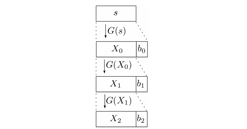
Pf. The main idea is using hybrid argument and contradiction. First we construct the recursive definition of \(G^{\prime}(s)=G^{m}(s)\) as
And define the hybrid distributions as
Thus
Assume there exists a distinguisher \(\mathsf{D}\) and a polynomial \(p(\cdot)\) such that for infinitely many \(n\), \(\mathsf{D}\) distinguishes \(\left\{U_{m(n)}\right\}_n\) and \(\left\{G^{\prime}\left(U_n\right)\right\}_n\) with probability \(\frac{1}{p(n)}\). Thus \(\mathsf{D}\) distinguishes \(H_n^0\) and \(H_n^{m(n)}\) with probability \(\frac{1}{p(n)}\). By the hybrid lemma, for each \(n\), there exists some \(i\) such that \(\mathsf{D}\) distinguishes \(H_{n}^{i}\) and \(H_{n}^{i+1}\) with probability \(\frac{1}{m(n) p(n)}\). Notice that
We consider the n.u. p.p.t. \(\mathsf{M}(y)\) whose output is \(U_{m-i-1}\left\|y_{1}\right\| G^{i}\left(y_{2}\cdots y_{n+1}\right)\). And \(\mathsf{M}(y)\) is non-uniform because for each \(n\), it needs the appropriate \(i\). We can discover that \(M\left(U_{n+1}\right)=H_n^i\) and \(M\left(G\left(U_{n}\right)\right)=H_{n}^{i+1}\). By the PRG property of \(G\), we have \(\left\{U_{n+1}\right\}_{n}\approx\left\{G(U_{n}))\right\}_{n}\), and by closure under efficient operations we can obtain that \(\left\{H_{n}^{i}\right\}_{n}\approx\left\{H_{n}^{i+1}\right\}_{n}\), this leads to a contradiction.
Hard-core bits
As long as we know that a PRG which extends the seed by only \(1\) bit can be used to create a PRG that extends an \(n\)-bit seed to \(\operatorname{poly}(n)\) output bits, we try to construct a predicate \(h\) that \(h(x)\) is next-bit unpredictable for the output bits \(f(x)\) of an one-way permutation \(f\). Then we have the definition for hardcore bit.
Def (Hard-core Predicate). A predicate \(h:\{0,1\}^*\rightarrow\{0,1\}\) is a hardcore bit for a one-way function \(f:\{0,1\}^{*}\rightarrow\{0,1\}^{*}\) if \(h\) is efficiently computable given \(x\) and for all p.p.t. adversary \(A\), there exists a negligible \(\eta(\cdot),\exists n_0\in N\), s.t. \(\forall n>n_0\),
Rem. As the way it is defined, a hardcore predicate \(h\) is defined relative to a one-way function \(f\), meaning that \(h\) may be a hardcore predicate for some one-way function \(f\), but not hardcore for other one-way functions.
Ex. We have two kinds of hardcore bits for RSA under the RSA assumption and one for discrete-log under the DL assumption.
-
The least significant bit of the RSA one-way function is known to be hardcore. Given \(N=pq,e\), and \(f_{N, e}(x)=x^{e}\bmod N\), here \(x=x_{n}\cdots x_{1}\). Then \(h(x)=\text{LSB}(x)=x_{1}\) is a hardcore bit for RSA.
-
The function \(\text{half}_{N}(x)\) is also hardcore for RSA, where
- The function \(\text{half}_{p-1}(x)\) is a hardcore predicate for exponentiation to the power \(x\bmod p\) (discrete-log) under the DL assumption.
Thm. If one-way permutation exists, PRG exists.
Pf. Let \(f\) be a one-way permutation and \(h\) be a hardcore predicate for \(f\) (we will see the existence of \(h\) later). Let \(G(x)=f(x)\|h(x)\). Since \(f\) is a permutation, \(f(x)\) is next-bit unpredictable clearly. Furthermore, \(h(x)\) is also unpredictable after see \(f(x)\). Thus \(G\) is a PRG.
Next, we are interested in the existence of hardcore bits. Unfortunately, there's no universal hardcore bit.
Thm. There is no function that is a hard-core bit of any OWF.
Pf. Suppose \(h\) is a such function, then \(f(x)h(x)\) should be an OWF, but \(h\) is not a hard-core bit for it obviously.
But... we have another kind of "universal" hard-core bit:
Thm (Goldreich and Levin, 1989). If \(f\) is a OWF, then for any n.u.p.p.t. \(A\), there exists a negligible function \(\epsilon(n)\) such that for all \(n \in \mathbb{N}\),
where \(\langle x, r \rangle\) is the inner product defined on \(\{0,1\}^n\):
Thus, the function \(f'(x\|r) = f(x)\|r\) is a OWF with a hardcore function \(h(x\|r) = \langle x, r \rangle\).
Pseudorandom Function
Def (Truly Random Function). A truly random function \(R_n:\{0,1\}^n\rightarrow\{0,1\}\) is a string consisting of \(2^{n}\) randomly generated bits. When we evaluate \(R_{n}\) on \(x\), \(R_{n}\) simply parse \(x\) as nonnegative integer \(0\leq t\leq 2^{n}-1\), and outputs the \(t+1\)-th bit in the string. More formally, let \(\mathsf{RF}_{n}=\{f:\{0,1\}^n\to\{0,1\}\}\), then a truly random function is obtained by uniformly generating from \(\mathsf{RF}_{n}\).
Def (Oracle Indistinguishability). Let \(\{O_n\}_{n\in\mathbb{N}}\) and \(\{O'_n\}_{n\in\mathbb{N}}\) be ensembles where \(O_n\), \(O'_n\) are probability distributions over functions \(f: \{0,1\}^{l_1(n)} \rightarrow \{0,1\}^{l_2(n)}\) for some polynomials \(l_1(\cdot)\), \(l_2(\cdot)\). We say that \(\{O_n\}_{n\in\mathbb{N}}\) and \(\{O'_n\}_{n\in\mathbb{N}}\) are computationally indistinguishable (denoted by \(\{O_n\}_n \approx \{O'_n\}_n\)) if for all non-uniform p.p.t. oracle machines \(\mathsf{D}\), there exists a negligible function \(\epsilon(\cdot)\) such that \(\forall n \in \mathbb{N}\):
Def (Pseudorandom Function). A family of functions \(\mathcal{F}=\left\{F_n=\{f_k: \{0,1\}^{n} \rightarrow \{0,1\}\}_{\mathcal{K}_n}\right\}_{n\in\mathbb{N}}\) is pseudorandom if:
-
\(|\mathcal{K}_n|\) is polynomial in \(n\).
-
\(f_k(x)\) can be computed by a p.p.t. algorithm given \(k\) and \(x\).
-
\(\{k \leftarrow \mathcal{K}_n : f_k\}_n \approx \{F \leftarrow \mathsf{RF}_{n} : F\}_n\).
Rem. We can generalize the definition of pseudorandom function to the case where \(f_{n, k}:\{0,1\}^{n}\rightarrow\{0,1\}^{\operatorname{poly}(n)}\) outputs a string rather than a single bit. In this case, we need to change the definition of truly random function so that it outputs random strings of length \(\text{poly}(n)\).
Thm. PRF exists iff PRG exists.
Pf. The direction \(\Rightarrow\) is easy:
Suppose \(\{f_k\}_{k\in\mathcal{K}_n}\) is a PRF. Construct \(g:\{0,1\}^n\to \{0,1\}^{m}\) as follows:
If there exists an adversary that can distinguish \(g(x)\) from random string, another adversary can send \(f(0)\|f(1)\|...\|f(m-1)\) to the former and distinguish \(f\) from random function.
For the other direction, [GGM86] offers a construction from PRG to PRF: Suppose \(G:\{0,1\}^n\to\{0,1\}^{2n}\) is a PRG. Split its output into two halves, yielding \(G^0, G^1: \{0,1\}^n \rightarrow \{0,1\}^n\) such that \(G(s) = G^0(s)\|G^1(s)\). Let the input be an \(n\)-bit string \(x = x_1...x_n\). Define:
resulting in:
which can be proved is a PRF.
Public Key Encryption
Concepts
Def (Public Key Encryption). A public key encryption scheme is a set of algorithms \((\mathsf{Gen},\mathsf{Enc},\mathsf{Dec})\) and the message space \(\mathcal{M}\) such that
-
The key Generation \(\mathsf{Gen}\) algorithm takes in a security parameter \(1^n\) and outputs \(\mathsf{Gen}(1^n) \to (pk,sk)\) where \((pk,sk)\) is a pair of public key and secret key.
-
The Encryption algorithm \(\mathsf{Enc}\) takes in the public key \(pk\) and a message \(m\in \mathcal{M}\) and outputs a ciphertext \(ct\), \(\mathsf{Enc}(pk, m) \to ct\).
-
The Decryption algorithm \(\mathsf{Dec}\) takes in the private key \(st\), the ciphertext \(ct\) and outputs the Decrypted message \(m'\) or \(\perp\) indicating that the input is invalid, \(\mathsf{Dec}(sk,ct) = m'/ \perp\).
Def (Correctness). A PKE is correct if \(\forall m\in \mathcal{M}\), we have
where \(\varepsilon(n)\) is negligible.
Rem. The probability is computed over all the randomness of \(\mathsf{Gen}\), \(\mathsf{Enc}\) and \(\mathsf{Dec}\). Even though the randomness of \(\mathsf{Enc}\) and \(\mathsf{Dec}\) is not shown explicitly in the definition, in general all the three algorithms can be probabilistic.
Def (Security). A PKE is secure if for any n.u.p.p.t. \(A\), there exists a negligible function \(\varepsilon\) such that \(\forall n \in \mathbb{N}\) and \(\forall m_0, m_1 \in \mathcal{M}\), we have
Constructing PKEs
First let's consider how to Encode a single bit.
Trapdoor permutations for PKE
We consider the following public key encryption scheme:
Let \(f_{N,a}(x)=x^{a}\pmod N\) be the RSA function. Suppose that \(h\) is a hardcore bit of \(f_{N,a}\), we construct the following scheme:
-
\(\mathsf{Gen}(1^n)\to p,q,\) which are used as secret keys
-
\(N=pq,a\leftarrow U(\Phi(N)),\) \(a\) and \(N\) are public keys
-
Find \(b\) s.t. \(ab=1\pmod{\Phi(N)},\) \(b\) is also the secret keys
-
\(\mathsf{Enc}(N,a,m)=f_{N,a}(r),h(r)\oplus m\) where \(r\leftarrow \mathbb{Z}_N^*\)
-
\(\mathsf{Dec}(f_{N,a}(r),h(r)\oplus m,b)\) can first find \(r=(f_{N,a}(r))^b\), then compute \(h(r)\) to recover \(m\)
The security of this scheme directly follows from the fact that \(h\) is a hardcore bit and we have that
given \(N\) and \(a\).
We can Generalize it for any trapdoor permutation:
- \(\mathsf{Gen}(1^n)=f_i,f_i^{-1}\), \(f_i\) and \(b_i\) are public key, \(f_i^{-1}\) is secret key
- \(\mathsf{Enc}(f_i,b_i,m)=f_i(r),b_i(r)\oplus m,\) where \(r\leftarrow \{0,1\}^n\)
- \(\mathsf{Dec}(f_i(r),b_i(r)\oplus m,f_i^{-1})\) can first find \(r=f_i^{-1}(f_i(r))\), then compute \(b_i(r)\) to recover \(m\)
Here, \((f_i,f^{-1})_{i\in I}\) is a family of one-way trapdoor permutations and \(b_i\) is the hard-core bit corresponding to \(f_i\).
Decisional Diffie-Hellman for PKE
We construct the following scheme for PKE:
- \(\mathsf{Gen}(1^n)=G,g\in G,|G|=p\)
- \(a\leftarrow \mathbb{Z}_p\) is the secret key, and the group \(G\), \(g^a\) and \(g\) are public
- \(\mathsf{Enc}(g,m)=mg^{ar},g^r\) where \(r\leftarrow \mathbb{Z}_p\)
- \(\mathsf{Dec}(a,mg^{ar},g^r,g)\) computes \((g^r)^a=g^{ar}\) and recover \(m\) by multiplying by \(g^{-ar}\)
where we let \(m\in G\) is a map from a bit to an non-zero element in \(G\).
To prove this, we apply the assumption that
where \(a,r,u\) are uniform.
Single bit to Multi bits
Here we proof that if we have a PKE scheme \((\mathsf{Gen}, \mathsf{Enc},\mathsf{Dec})\) that encodes a single bit \(b\) such that for any n.u.p.p.t. adversary \(\mathcal{A}\) we have
for all \(n \in \mathbb{N}\) and \(\epsilon\) is negligible. Then for polynomially long messages \(m_0, m_1\), we have a PKE scheme \((Gen,\mathsf{Enc}',\mathsf{Dec}')\) such that for all n.u.p.p.t. \(\mathcal{A}\), we have
here we let \(\mathsf{Enc}'\) be the algorithm that encodes the message \(m\) bit-by-bit using \(\mathsf{Enc}\) and similarly for \(\mathsf{Dec}'\).
Suppose on the contrary that there exists a n.u.p.p.t. \(\mathcal{A}\) such that for infinitely many \(n \in \mathbb{N}\), there exist \(2\) messages \(m_0, m_1 \in \mathcal{M}\) such that
for a polynomial \(p\). We construct a hybrid argument using the following strings
where \(m = \mathsf{poly}(n)\). It is clear that \(m^H_0 = m_1\) and \(m^H_m = m_0\). Consequently we see that there exists \(j\) such that
where \(m^H_j\) and \(m^H_{j+1}\) only differ in the \(j+1\)th bit. Hence the \(j+1\)th bit of \(m_0\) and \(m_1\) must be different.
Now we construct the following n.u.p.p.t. \(\mathcal{A}'\) (note that \(\mathcal{A}'\) has \(j\) and \(m_0, m_1\) hardcoded)
-
\(\mathsf{Gen}(1^n) \rightarrow (pk, sk)\)
-
On input \(\mathsf{Enc}(pk, b), b \in \{0, 1\}\), \(\mathcal{A}'\) encodes the first \(j\) bits of \(m_0\) using \(\mathsf{Enc}'\) and the \(j+2\)th to \(m\)th bits of \(m_1\) using \(\mathsf{Enc}'\), and inputs \(\mathsf{Enc}'(pk, m_0[1:j])||\mathsf{Enc}(pk, b)||\mathsf{Enc}'(pk, m_1[(j+2):m])\) to \(\mathcal{A}\)
\(\mathcal{A}'\) returns the output of \(\mathcal{A}\)
and it is easily seen that
for infinitely many \(n \in \mathbb{N}\), which is a contradiction.
Secret Key Encryption
Concepts
Def (Secret Key Encryption). A secret key encryption (SKE) is a set of algorithms \((\mathsf{Gen}, \mathsf{Enc}, \mathsf{Dec})\) and a message space \(\mathcal{M}\), where:
- \(\mathsf{Gen}(1^n) \to sk\)
- \(\mathsf{Enc}(sk, m) \to ct\)
- \(\mathsf{Dec}(sk, ct) \to {m, \perp}\) (\(\perp\) means failed).
Def (Correctness of SKE). An SKE scheme is correct if there exists a negligible function \(\varepsilon(n)\), for all \(m \in \mathcal{M}\), $$\Pr[\mathsf{Dec}(sk, \mathsf{Enc}(sk, m)) = m] \geqslant 1 - \varepsilon(n)$$ over all the randomness.
Now let's consider how to define the security of SKE. Here are some attempts:
Attempt 1. \(\forall\) non-uniform polynomial-time (n.u.p.p.t.) \(A\), \(\exists\) negligible function \(\varepsilon(n)\), such that \(\forall n \in \mathbb{N}, \forall m_0, m_1 \in \mathcal{M}\): $$\left| \Pr[sk \gets \mathsf{Gen}, A(1^n, \mathsf{Enc}(sk, m_0)) = 1] - \Pr[sk \gets \mathsf{Gen}, A(1^n, \mathsf{Enc}(sk, m_1)) = 1] \right| < \varepsilon(n)$$ Can we reuse the key to encrypt multiple messages?
Recall \(\mathsf{Enc}\) uses only \(pk\) to encrypt the message in PKE.
Attempt 2. \(\forall\) n.u.p.p.t. \(A\), \(\exists\) negligible function \(\varepsilon(n)\), such that \(\forall n \in \mathbb{N}, \forall (m_0^{(1)}, m_0^{(2)}, \dots, m_0^{(L)}), (m_1^{(1)}, m_1^{(2)}, \dots, m_1^{(L)}) \in \mathcal{M}^L\) where \(L\) is a polynomial of \(n\): $$\left| \Pr[sk \gets \mathsf{Gen}, A(1^n, \mathsf{Enc}(sk, m_0^{(1)}), \dots, \mathsf{Enc}(sk, m_0^{(L)})) = 1] - \Pr[sk \gets \mathsf{Gen}, A(1^n, \mathsf{Enc}(sk, m_1^{(1)}), \dots, \mathsf{Enc}(sk, m_1^{(L)})) = 1] \right| < \varepsilon(n)$$
Attempt 3. Use \(\mathsf{Enc}\) as an oracle. This attempt directly leads to the following definition:
Def (SKE secure against chosen plaintext attack, CPA secure). Consider a game between a game master Eve and a challenger as follows:
- Challenger generates \(sk\) at first.
- Eve sends \(m\), and challenger returns \(\mathsf{Enc}(sk, m)\) for \(\text{poly}(n)\) turns.
- Eve sends \(m_0, m_1\). Then challenger chooses \(b \in \{0,1\}\) and returns \(\mathsf{Enc}(sk, m_b)\). (Challenge phase.)
- Eve sends \(m\), and challenger returns \(\mathsf{Enc}(sk, m)\) for \(\text{poly}(n)\) turns.
- Eve sends \(b'\), and wins if and only if \(b = b'\).
The SKE scheme is semantically secure under chosen plaintext attack if \(\forall\) n.u.p.p.t. \(A\), \(\exists\) negligible function \(\varepsilon(n)\), such that \(\forall n \in \mathbb{N}\): $$\Pr_{\text{all the randomness}}[A \text{ wins the CPA game}] < \frac{1}{2} + \varepsilon(n)$$ Rem. Note that \(\mathsf{Enc}\) must depend on some randomness in this definition. Otherwise, the adversary can just query \(m_0, m_1\) and then compare their results.
There are several proposed changes to this definition:
- Can we fix the value of \(m_0\) and \(m_1\) at first? Note that Eve can choose \(m_0\) and \(m_1\) adaptively.
- Can we fix the queries at first?
- Can the adversary call \(\mathsf{Dec}\)?
Attempt 4. Use both \(\mathsf{Enc}\) and \(\mathsf{Dec}\) as an oracle.
Def (SKE secure against chosen ciphertext attack, CCA secure). Consider a game between a game master Eve and a challenger as follows:
- Challenger generates \(sk\) at first.
- Eve sends \(m, c\), and challenger returns \(\mathsf{Enc}(sk, m), \mathsf{Dec}(sk, c)\) for \(\text{poly}(n)\) turns.
- Eve sends \(m_0, m_1\). Then challenger chooses \(b \in \{0,1\}\) and returns \(\mathsf{Enc}(sk, m_b)\). (Challenge phase.)
- Eve sends \(m, c\), and challenger returns \(\mathsf{Enc}(sk, m), \mathsf{Dec}(sk, c)\) for \(\text{poly}(n)\) turns.
- Eve sends \(b'\), and wins if and only if \(b = b'\).
The SKE scheme is semantically secure under chosen ciphertext attack if \(\forall\) n.u.p.p.t. \(A\), \(\exists\) negligible function \(\varepsilon(n)\), such that \(\forall n \in \mathbb{N}\): $$\Pr_{\text{all the randomness}}[A \text{ wins the CCA game}] < \frac{1}{2} + \varepsilon(n)$$ Rem. What if the adversary queries \(\mathsf{Dec}(\mathsf{Enc}(sk, m_b))\)? Several remedies:
- CCA1: Can only ask \(\mathsf{Dec}\) queries before challenge phase.
- CCA2: Can ask anything except for \(\mathsf{Enc}(sk, m_b)\).
Constructing Secure SKEs from PRF
Thm. If PRF exists, CPA secure SKE exists.
Pf. Let \(\mathcal{F} = \{F^n = \{f_k^n : \{0,1\}^n \to \{0,1\}^n\}_{k \in \mathcal{K}^n}\}\) be a PRF family. And the length of \(m\) is \(n\). Consider the following SKE:
- \(\mathsf{Gen}(1^n) \to k \in \mathcal{K}^n\)
- \(\mathsf{Enc}(k, m) \to (f_k^n(r) \oplus m, r)\) where \(r \gets \{0,1\}^n\), let \(ct_1 = f_k^n(r) \oplus m\) and \(ct_2 = r\).
- \(\mathsf{Dec}(k, (ct_1, ct_2)) \to ct_1 \oplus f_k^n(ct_2)\)
Why does this construction satisfy CPA secure? Hybrid Lemma!
Consider the following three CPA games, with only different encode function:
- Real world:
- When Eve sends \(m^{(i)}\), and challenger returns \(f_k^n(r^{(i)}) \oplus m^{(i)}, r^{(i)}\), where \(r^{(i)} \leftarrow \{0,1\}^n\).
- When Eve sends \(m_0, m_1\). Then challenger chooses \(b \in \{0,1\}\) and returns \(f_k^n(r^*) \oplus m_b, r^*\), where \(r^* \leftarrow \{0,1\}^n\).
- Hybrid 1:
- When Eve sends \(m^{(i)}\), and challenger returns \(R^{(i)} \oplus m^{(i)}, r^{(i)}\), where \(R^{(i)}, r^{(i)} \leftarrow \{0,1\}^n\).
- When Eve sends \(m_0, m_1\). Then challenger chooses \(b \in \{0,1\}\) and returns \(R^* \oplus m_b, r^*\), where \(R^*, r^* \leftarrow \{0,1\}^n\).
- Hybrid 2:
- When Eve sends \(m^{(i)}\), and challenger returns \(R^{(i)}, r^{(i)}\), where \(R^{(i)}, r^{(i)} \leftarrow \{0,1\}^n\).
- When Eve sends \(m_0, m_1\). Then challenger chooses \(b \in \{0,1\}\) and returns \(R^*, r^*\), where \(R^*, r^* \leftarrow \{0,1\}^n\).
Since you can't get any information of \(b\) in hybrid 2, Eve always loses with probability \(\frac{1}{2}\). Also, hybrid 1 and hybrid 2 are perfectly indistinguishable clearly. So we only need to prove that hybrid 1 is computationally indistinguishable from real world, according to the properties of PRF.
Suppose this scheme is not CPA secure, that is, there exists a n.u.p.p.t. adversary \(A\) such that there is a non-negligible function \(\delta(n)\), $$\left| \Pr[A^{\text{real world with } b=0}(1^n) = 1] - \Pr[A^{\text{real world with } b=1}(1^n) = 1] \right| \ge \delta(n).$$ On the other hand, $$\left| \Pr[A^{\text{hybrid 1 with } b=0}(1^n) = 1] - \Pr[A^{\text{hybrid 1 with } b=1}(1^n) = 1] \right| = 0.$$ Thus, there exists \(c \in \{0,1\}\) such that $$\left| \Pr[A^{\text{real world with } b=c}(1^n) = 1] - \Pr[A^{\text{hybrid 1 with } b=c}(1^n) = 1] \right| \ge \frac{\delta(n)}{2}.$$ Then we construct \(B\) to distinguish \(F_k(\cdot)\) from a truly random function \(R(\cdot)\) as follows. Let \(O(\cdot)\) either be \(F_k(\cdot)\) or \(R(\cdot)\).
\(B\) starts a CPA game. When \(A\) queries \(m^{(i)}\), \(B\) picks \(r^{(i)} \gets \{0,1\}^n\), and queries \(r^{(i)}\), getting \(y = O(r)\). Then \(B\) sends \(O(r^{(i)}) \oplus m, r^{(i)}\) back to \(A\). When \(A\) queries \(m_0, m_1\), \(B\) picks \(r^* \gets \{0,1\}^n\), and queries \(r^*\), getting \(y^* = O(r^*)\). Then \(B\) sends \((O(r^*) \oplus m_c, r^*)\) back to \(A\). Finally, \(B\) returns the same value as \(A\).
Thus
This leads to a contradiction. Thus such adversary \(A\) doesn't exist.
Rem. What if the expected running time of the adversary is polynomial, but sometimes it runs in exponential time? In this case, the number of hybrids may be exponential, which is not acceptable.
Def (weak PRF). If the adversary is only allowed to make random queries in the definition of a PRF, we call it a weak PRF.
Thm. If weak PRF exists, CPA secure SKE exists.
Pf. In the above construction, all the oracle queries have random input. This immediately gives the result.
In fact, such construction is also CCA1 secure.
Thm. If PRF exists, CCA1 secure SKE exists.
Besides, we have the following result:
Thm. If PRF exists, CCA2 secure SKE exists.
Pf. Let \(\mathcal{F} = \{F^n = \{f_k^n : \{0,1\}^n \to \{0,1\}^n\}_{j \in \mathcal{J}^n}\}\) and \(\mathcal{G} = \{G^n = \{g_k^n : \{0,1\}^n \to \{0,1\}^n\}_{k \in \mathcal{K}^n}\}\) be PRF families. And the length of \(m\) is \(n\). Consider the following SKE:
- \(\mathsf{Gen}(1^n) \to j \in \mathcal{J}^n, k \in \mathcal{K}^n\)
- \(\mathsf{Enc}(j, k, m) \to (r, ct_1, ct_2)\) where \(r \gets \{0,1\}^n, ct_1 = m \oplus f_j^n(r), ct_2 = g_k^n(ct_1)\).
- \(\mathsf{Dec}(j, k, (r, ct_1, ct_2)) \to ct_1 \oplus f_j^n(r)\) if \(ct_2 = g_k^n(ct_1)\), \(\perp\) otherwise.
We can show that the above SKE is CCA2 secure.
Knowledge
Simulation Paradigm
We learned about the definition of CPA security, which is an indistinguishability-based definition of security.
Def (ind-based definition scheme (Informal)). An encryption scheme is CPA secure if \(\mathsf{Enc}_{k}(0)\) and \(\mathsf{Enc}_{k}(1)\) are computationally indistinguishable.
In this lecture, we introduce a different definition of security, which is simulation-based.
Intuitively, we consider a scenario as follows: you are an adversary, and you have seen many ciphertexts, but you gain no knowledge from the message, it can explained as that there is a real world in which you receive a ciphertext, and there is also an ideal world in which a p.p.t simulator with no more knowledge than you about the secret key of generating fake message, but you can not distinguish the texts from two world as an adversary.
Def (simulation-based encryption scheme). An encryption scheme is a simulation secure scheme, if there exists a p.p.t. simulator \(S\) such that, for all n.u. p.p.t. \(A\), there exists a negligible function \(\epsilon(n)\), such that \(\forall n>n_{0}\) and for all auxiliary information \(z,\forall m\in \mathcal{M}\)
Def (zero-knowledge encryption scheme). A private-key encryption scheme is a zero-knowledge encryption scheme, if there exists a p.p.t simulator \(S\) such that, for all n.u. p.p.t \(A\), there exists a negligible function \(\epsilon(n)\), such that \(\forall m\in\mathcal{M}\) it holds that \(A\) distinguishes the following distributions with probability at most \(\epsilon(n)\)
- \(\left\{k\leftarrow\mathsf{Gen}\left(1^{n}\right): \mathsf{Enc}_{k}(m)\right\}\)
- \(\left\{S\left(1^{n}\right)\right\}\)
Rem. Intuitively the simulation-based definition is stricter than the zero-knowledge definition. But we will see they are equivalent. We introduce the notion of auxiliary information because it will be useful later when we introduce zero-knowledge proof.
Rem. For simplicity, in the following of notes, we choose \(\mathcal{M}=\{0,1\}\), this is not necessary but simplify our argument.
Ex. Let \(F=\{f_k:\{0,1\}^n\to\{0,1\}\}_k\) be a PRF. Consider the following encryption scheme:
- \(\mathsf{Gen}(1^n)\to k\)
- \(\mathsf{Enc}_k(m)\to \left(r, t=f_{k}(r)\oplus m\right)\), where \(m\gets \{0,1\},r\gets\{0,1\}^n\)
- \(\mathsf{Dec}_k(r,t)\to m=f_{k}(r)\oplus t\)
We already show that it's ind-based secure. Now let's show that it's also simulation-based secure.
Pf. Construct simulator \(S\): sample \(r_{\text{sim}}\leftarrow\{0,1\}^{n}, t_{\text{sim}}\leftarrow\{0,1\}\), output \(r_{\text{sim}}, t_{\text{sim}}\). If there exists a n.u.p.p.t adversary \(A\) and auxiliary information \(z\) that can distinguish \(\mathsf{Enc}_k(m)\) and \(\left(r_{\text{sim}}, t_{\text{sim}}\right)\) with non-negligible probability, then consider n.u.p.p.t \(A^{\prime}(1^n,r, x)=A\left(1^{n},(r, x\oplus m), z\right)\) can distinguish \(\left(r, f_{k}(r)\right)\) and \((r, U_1)\) with non-negligible probability, which leads to a contradiction.
Now let's show that the three definitions of security are equivalent.
Thm. Let \(\mathsf{(Gen, Enc, Dec)}\) be an private key encryption scheme, then ind-secure is equivalent to simulation-secure and is equivalent to zero-knowledge.
Pf. We break the proof into three parts.
-
ind-secure \(\Rightarrow\) simulation-secure
Suppose \(\mathsf{(Gen, Enc, Dec)}\) is ind-secure but not simulation-secure. We can build a following simulator \(S(1^{n})\):
- \(k\gets \mathsf{Gen}(1^n)\)
- Output \(c=\mathsf{Enc}_k(0)\)
Then by assumption, \(\exists\) n.u.p.p.t. \(A\), auxiliary information \(z\) and a polynomial \(p(n)\) s.t., for infinitely many \(n\), there exists message \(m\) s.t.,
\[\left|\mathsf{Pr}\left[k\gets \mathsf{Gen}(1^n):\mathsf{A}\left(1^{n},\mathsf{Enc}_{k}(m), z\right)=1\right]-\mathsf{Pr}\left[k\gets \mathsf{Gen}(1^n):\mathsf{A}\left(1^{n},\mathsf{Enc}_{k}(0), z\right)=1\right]\right|\geq\frac{1}{p(n)}. \]Clearly it must holds \(m=1\). Then consider n.u.p.p.t. \(A^{\prime}\left(1^{n}, x\right)=A\left(1^{n}, x, z\right)\) and \(A^{\prime}\) can distinguish \(\mathsf{Enc}_{k}(1)\) and \(\mathsf{Enc}_{k}(0)\) with non-negligible probability, contradicting the definition of ind-based security.
-
simulation-secure \(\Rightarrow\) zero-knowledge
In the definition of simulation-secure, we can choose \(z\) to empty string and get the definition of zero-knowledge.
-
zero-knowledge \(\Rightarrow\) ind-secure
If the encryption scheme is zero-knowledge, we can use hybrid argument to show the following distribution are computationally indistinguishable.
- \(\left\{k\leftarrow\mathsf{Gen}\left(1^{n}\right):\mathsf{Enc}_{k}(0)\right\}\)
- \(\left\{S\left(1^{n}\right)\right\}\)
- \(\left\{k\leftarrow\mathsf{Gen}\left(1^{n}\right):\mathsf{Enc}_{k}(1)\right\}\)
Zero-Knowledge Proofs
Interactive Proofs
An interactive proof system contains a prover \(P\) and a verifier \(V\). The prover and the verifier will send messages in turns for a polynomial number of times.
Here is an example of interactive proof to solve the graph non-isomorphism problem.
Def (Graph Isomorphism). Given two graphs \(G_{1} = \left(V_{1}, E_{1}\right), G_{2} = \left(V_{2}, E_{2}\right)\). Suppose \(\left|V_{1}\right| = \left|V_{2}\right| = n\). We say that \(G_{1}\) and \(G_{2}\) are isomorphic (or \(G_{1} \cong G_{2}\)) if \(\exists \pi \in \Pi_{n}, \pi\left(G_{1}\right) = G_{2}\).
Here \(\pi\) is a permutation. \(\pi(G) = \left(\left\{\pi\left(v_{i}\right), v_{i} \in V\right\}, \left\{\left(\pi\left(v_{i}\right), \pi\left(v_{k}\right)\right), \left(v_{i}, v_{j}\right) \in E\right\}\right)\)
The interactive proof of graph non-isomorphism is following:
- \(x = \left(G_{1}, G_{2}\right)\)
- Verifier: Randomly sample \(b \leftarrow \{1,2\}, \pi \leftarrow \Pi_{n}\). Send \(\pi\left(G_{b}\right)\).
- Prover: Send \(b^{\prime}\) such that \(G_{b^{\prime}} \cong \pi\left(G_{b}\right)\).
- Verifier: Check if \(b^{\prime} = b\).
- Repeat 2,3,4.
If \(G_{1}, G_{2}\) are not isomorphic, a prover with unlimited power can find \(b^{\prime}\) for any \(b, \pi\).
If \(G_{1}, G_{2}\) are isomorphic, however, \(\pi\left(G_{b}\right)\) is isomorphic with both \(G_{1}\) and \(G_{2}\). Since \(\pi\) is randomly chosen, \(b\) can be \(1\) or \(2\) with equal probability. Thus, even a computationally unbounded can only find \(b^{\prime} = b\) with probability \(1/2\).
Now we formally define the interactive proof system.
Protocol. For a certain language \(L\), we want to determine if an instance \(x\in L\), and there is a prover \(P(x, y)\) taking \(x\) and witness \(y\) as input, a verifier \(V(x, z)\) taking \(x\) and an auxiliary information \(z\) as input. The execution goes as:
- In the \(i^{\text{th}}\) round, the prover sends \(\alpha_{i}\) to the verifier, the verifier sends \(\beta_{i}\) to the prover;
- The execution runs for \(k\in\mathsf{poly}(n)\) rounds. Then the verifier accepts \(x\) or rejects \(x\) depending on the transcripts \(\left(\alpha_{1},\beta_{1},\ldots,\alpha_{k},\beta_{k}\right)\) and this execution ends.
Denoted the execution as \(P(x,y)\leftrightarrow V(x,z)\). For a certain execution \(e\), denote the information output by \(X\) in \(e\) as \(\text{out}_X[e]\), and all the information viewed by \(X\) as \(\text{view}_X[e]\).
Def (Interactive Proof System). \((P,V)\) is an interactive proof system for \(L\) if
-
(Completeness) \(\forall x \in L\), the prover \(P(x)\) (computationally unbounded) can convince the verifier \(V\) (in polynomial time) with a probability \(1\), that is, there exists a witness string \(y\in\{0,1\}^*\) such that for every auxiliary string \(z\):
\[\text{Pr}[\text{out}_V[P(x,y)\leftrightarrow V(x,z)]=1]=1. \] -
(Soundness) \(\forall x \notin L\), for all computationally unbounded prover \(P^*, P^*\) can convince the verifier \(V\) (in polynomial time) with a probability less than \(\frac{1}{2}\), that is, for all auxiliary string \(z\):
\[\text{Pr}[\text{out}_V[P^*(x)\leftrightarrow V(x,z)]=0]>\frac{1}{2}. \]
Rem. In different definitions of interactive proof system, the latter probability "\(\frac{1}{2}\)" may be replaced with "\(1-\epsilon\)".
Zero-Knowledge Proofs
Now we consider zero-knowledge proofs in which the prover wants to "convince" the verifier without revealing any additional information. Before strictly defining zero-knowledge proofs, we provide a zero-knowledge proof algorithm for the graph isomorphism (GI) problem.
Zero-Knowledge Proof for the Graph Isomorphism Problem
Suppose that \(\pi\left(G_{1}\right) = G_{2}\), where \(\pi\) is unknown to the verifier. The prover wants to convince the verifier that \(\pi\) exists without providing any additional information about \(\pi\).
This can be done with the following steps:
- The prover randomly selects some permutation \(\sigma \in \Pi_{n}\), and sends \(G^{\prime} = \sigma\left(G_{1}\right)\) to the verifier.
- The verifier randomly selects some \(b \in \{1,2\}\), and sends \(b\) to the prover.
- If \(b = 1\), the prover sends \(\pi^{\prime} = \sigma\) to the verifier. If \(b = 2\), then the prover sends \(\pi^{\prime} = \sigma \circ \pi^{-1}\).
- The verifier verifies whether \(G^{\prime} = \pi^{\prime}\left(G_{b}\right)\).
- Repeat the above process several times.
We now show why the verifier should be convinced in this way. Suppose \(G_{1}\) are \(G_{2}\) are not isomorphic. In this case, \(G^{\prime}\) is isomorphic to at most one of \(G_{1}\) and \(G_{2}\). Since \(b\) is randomly chosen by the verifier, the probability that \(G^{\prime}\) is isomorphic to \(G_{b}\) is at most \(1/2\). Thus, despite the fact that the prover may violate the protocols, it cheats the verifier with probability at most \(1/2\). On the other hand, if \(G_{1}\) and \(G_{2}\) are isomorphic, then \(G^{\prime}\) will always be identical with \(\pi^{\prime}\left(G_{b}\right)\).
Since \(\sigma\) is randomly chosen and unknown to the verifier, intuitively, the verifier cannot discover any additional information about \(\pi\) from \(\pi^{\prime}\), as long as graph isomorphism is hard.
Formal Definition
Now we move on to formally define what is a zero-knowledge interactive proof system. Intuitively, the fact that the verifier gets no additional information means that the whole process of interactive proving is indistinguishable from what the verifier itself can derive. Thus, we can define zero-knowledge interactive proof system as follows.
Def (Zero-Knowledge Interactive Proof System). \((P, V)\) is a zero-knowledge interactive proof system for \(L\) if
-
(Completeness) \(\forall x \in L\), the prover \(P\) (computationally unbounded) can convince the verifier \(V\) (in polynomial time) with probability \(1\).
-
(Soundness) \(\forall x \notin L\), for all computationally unbounded prover \(P^{*}, P^{*}\) can convince the verifier \(V\) (in polynomial time) with probability less than \(\frac{1}{2}\).
-
(Zero-knowledge for honest verifier) there exists a witness string \(y\) and p.p.t. \(S\) such that \(\forall z \in \{0,1\}^{*}\),
\[\{S(x,z)\}\approx\{\text{view}_V[P(x,y)\leftrightarrow V(x,z)]\} \]
Rem. One concept to notice is "honest verifier". This intuitively means that the verifier will strictly follow the proof protocol. For example, consider step 2 in the zero-knowledge proof algorithm for the GI problem, an honest verifier will always choose \(b\) randomly. On the other hand, a malicious verifier may choose \(b\) based on some carefully chosen strategy such that it can "steal" some information from the prover.
Now let's show the above protocol for GI is zero-Knowledge for honest verifier. Just construct a p.p.t simulator \(S\) for this scenario:
- The prover in \(S\), say \(P^{S}\), generates \(\sigma^{S}\in\Pi_{n}\) and \(b^{S}\in\{0,1\}\) randomly and sends \(H^{S}=\) \(\sigma^{S}\left(G_{b}^{S}\right)\) to the verifier in \(S\), say \(V^{S}\);
- \(V^{S}\) sends back \(b\) to \(P^{S}\);
- \(P^{S}\) sends back \(\pi^{\prime}=\sigma^{S}\);
- Repeat the steps above several times.
Def (Zero-Knowledge Interactive Proof System for a Malicious Verifier). \((P, V)\) is a zero-knowledge interactive proof system for \(L\) if
-
(Completeness) \(\forall x \in L\), the prover \(P\) (computationally unbounded) can convince the verifier \(V\) (in polynomial time) with probability \(1\).
-
(Soundness) \(\forall x \notin L\), for all computationally unbounded prover \(P^{*}, P^{*}\) can convince the verifier \(V\) (in polynomial time) with probability less than \(\frac{1}{2}\).
-
(Zero-knowledge for malicious verifier) For any p.p.t. \(V^*\), there exists a witness string \(y\) and p.p.t. \(S\) such that \(\forall z \in \{0,1\}^{*}\),
\[\{S(x,z)\}\approx\{\text{view}_{V^*}[P(x,y)\leftrightarrow V^*(x,z)]\} \]e.g. \(S\) may know the program of \(V^{*}\).
Rem. There are three levels for zero-knowledge, depends on how '\(\approx\)' defined. \(S\) can be under the different conditions depends on different '\(\approx\)':
- \(\approx_{o}\) is perfect ZK: \(S\) runs in expect p.p.t.;
- \(\approx_{o}\) is statistical/computational ZK: \(S\) runs in p.p.t.
Ex. For a simulator \(S\) for \(V^{*}\) in above GI problem:
- \(\beta_{1}: b^{S}\in\{0,1\}\).
- \(\alpha_{2}:\Pi^{\prime S}\in\Pi_{n}\).
- \(\alpha_{1}: H^{S}=\Pi^{\prime S}\left(G_{b^{S}}\right)\).
- \(b^{\prime}:\) Run \(V^{*}\) on \(H^{S}, b^{\prime}=V^{*}\left(H^{S}\right)\).
- If \(b^{\prime}=b^{S}\), output \(\left(H^{S}, b^{S},\Pi^{\prime S}\right)\) as \(\left(\alpha_{1},\beta_{1},\alpha_{2}\right)\); If \(b^{\prime}\neq b^{S}\), goto 1;
Notice that for all \(V^{*},\text{Pr}\left[b^{\prime}=b^{S}\right]=\frac{1}{2}\), \(S\) would finish with probability \(\frac{1}{2}\) in every loops. \(\left\{\text{view}_{V^{*}}[P\leftarrow V^*]\right\}\approx_{o}\left\{S(x, z)\right\}\), so the proof is zero-knowledge for a malicious verifier.
Rem. GI belongs to PZK with a simulator that runs in expected polynomial time, and GI belongs to SZK with a simulator that runs in strict polynomial time.
Authentication
Digital Signatures
Def. A digital signature scheme is a tuple of three p.p.t. algorithms \((\mathsf{Gen}, \mathsf{Sign}, \mathsf{Ver})\):
-
\(\mathsf{Gen}(1^{n})\rightarrow(sk, vk)\), where \(sk\) is the secret key and \(vk\) is the verification key.
-
\(\mathsf{Sign}(sk, m)\rightarrow\sigma\), the signature of the message based on secret key \(sk\) and message \(m\).
-
\(\mathsf{Ver}(vk, m,\sigma)\rightarrow\) \(0/1\), indicating whether \(\sigma\) is the signature for \(m\), based on verification key \(vk\).
-
(Correctness) For all \(n\in \mathbb{N}\) and \(m\in \mathcal{M}_n\),
\[\text{Pr}[sk,vk\leftarrow \mathsf{Gen}(1^n),\sigma\leftarrow \mathsf{Sign}(sk,m):\mathsf{Ver}(vk,m,\sigma)=1]=1. \]
Def. \((\mathsf{Gen}, \mathsf{Sign}, \mathsf{Ver})\) is a secure digital signature scheme if for all n.u. p.p.t. adversaries \(A\), there exists a negligible function \(\epsilon(n)\), such that for all \(n\in\mathbb{N}\),
In other words, \(A\) only has a negligible probability of winning the Forgery Game:
Def (Forgery Game). In the forgery game there are two parties, challenger \(\mathsf{C}\) and adversary \(A\). The game runs as follows:
- \(\mathsf{C}\) computes \(\mathsf{Gen}\left(1^{n}\right)\to(sk, vk)\), and send \(vk\) to \(A\).
- \(A\) sends \(m_{1}\) to \(\mathsf{C}\), and obtains \(\sigma_{1}=\mathsf{Sign}\left(m_{1}, sk\right)\) in response.
- \(A\) and \(\mathsf{C}\) repeat step 2 for multiple times, in round \(i\), \(A\) sends \(m_{i}\) to \(\mathsf{C}\), and receives \(\sigma_{i}\).
- \(A\) sends \(\left(m^{*},\sigma^{*}\right)\) to \(\mathsf{C}\).
\(A\) wins if:
- \(\mathsf{Verify}\left(m^{*},\sigma^{*}\right)=1\)
- \(m^{*}\) has not been queried before.
Ex. Consider a DS with verification algorithm \(\mathsf{Ver}(vk,m,\sigma)\) as follows: check whether
for some function family \(\{f_{vk}\}_{vk}\). It's straightforward that such DS cannot be secure since we can pick random \(\sigma\) and let \(m=f_{vk}(\sigma)\).
Rem. This example shows that a secure DS must based on some computational hardness on inverting \(\mathsf{Ver}\).
Constructing DS
Thm. If OWF exists, DS exists.
Pf. See [Rompel 90].
Since this results is too complex, let's see some easier case.
Constructing DS from RO
Def (Random Oracle Model). The random oracle model is the assumption of the existence of a hash function \(\mathcal{H}\) that "behaves" like a truly random function. Formally, for any p.p.t. adversary \(A\), given oracle access to \(\mathcal{H}\) or a truly random function, \(A\) should not distinguish whether the oracle it has is a truly random function or \(\mathcal{H}\).
Rem. The random oracle model cannot be true, since for a fixed \(\mathcal{H}\), adversary can just select input \(x_0\) and evaluate \(\mathcal{H}\left(x_{0}\right)\), then adversary can just query the oracle on \(x_{0}\) to see if the values fit.
We can view the random oracle as a trusted party \(\mathcal{O}\). Everybody in the world can query \(\mathcal{O}\) on any input \(x\). For every query \(x\), \(\mathcal{O}\) will respond using a random answer. Also, \(\mathcal{O}\) will always give the same response when queried on the same input.
When constructing DS schemes, we can allow the algorithms \(\mathsf{Sign}\) and \(\mathsf{Ver}\) to query the trusted party \(\mathcal{O}\). However, in reality we don't have such a magical party, and the random oracle model states that we can replace the party \(\mathcal{O}\) with a hash function \(\mathcal{H}\) with "reasonably" good property, and if the DS scheme (or other schemes that we need to use random oracle to construct) is secure when random oracle exists, we are confident that after we replace \(\mathcal{O}\) with \(\mathcal{H}\), the scheme is still secure enough.
Thm. Assume \(\mathcal{H}\) is a hash function with "reasonably good" property. Then the following is a DS scheme that is correct and secure in the random oracle model:
- \(\mathsf{Gen}\left(1^{n}\right)\): Generate two primes \(p,q\) of length \(n\) (i.e., \(2^{n-1}\leq p, q<2^{n}\)), set \(N=p q\). Randomly sample \(d\leftarrow \mathbb{Z}_{\phi(N)}^{*}\) and compute \(e\equiv d^{-1}\pmod{\phi(N)}\). Output \((sk, vk)\) with \(sk=(d, N), vk=(e,N)\).
- \(\mathsf{Sign}(sk, m)\): Just compute \(\sigma=(\mathcal{H}(m))^{sk}\bmod N\).
- \(\mathsf{Verify}(vk, m,\sigma)\): Checks if \(\sigma^{vk}\equiv\mathcal{H}(m)\pmod N\), if so, output \(1\), otherwise output \(0\).
A One-Time Signature Scheme
A digital signature scheme is said to be one-time secure if the definition is satisfied under the constraint that the adversary \(A\) is only allowed to query the signing oracle once.
Thm. If OWF exists, one-time secure DS exists.
Pf. Let \(f:\{0,1\}^n\to\{0,1\}^n\) be a one-way function. Consider the following scheme:
-
\(\mathsf{Gen}(1^n)\): For \(i=1,...,n\), and \(b=0,1\), pick \(x_b^i\leftarrow U_n\). Output the keys:
\[sk=(x_0^1,...,x_0^n,x_1^1,...,x_1^n),\\ vk=(f(x_0^1),...,f(x_0^n),f(x_1^1),...,f(x_1^n)). \] -
\(\mathsf{Sign}(sk,m)\): For \(i=1,...,n\), let \(\sigma_i=x_{m_i}^i\), output \(\sigma=(\sigma_1,...,\sigma_n)\).
-
\(\mathsf{Ver}(vk,\sigma,m)\): Output \(1\) iff \(f(\sigma_i)=f(x^i_{m_i})\) for all \(i=1,...,n\).
Let's show this construction is one-time secure. By contradiction. Suppose we are given an adversary \(A\) that succeeds with probability \(\epsilon(n)\) in breaking this signature scheme. We construct a new adversary \(B\) that inverts \(f\) with probability \(\frac{\epsilon(n)}{2n}\).
Let \(m\) and \(m'\) be the two messages chosen by \(A\) (\(m\) is \(A\)'s request to the signing oracle, and \(m'\) is in \(A\)'s output). \(B\) generates an instance of \((\mathsf{Gen}, \mathsf{Sign}, \mathsf{Ver})\) using \(f\) and replaces one of the values in \(pk\) with \(y\). With some probability, \(A\) will choose a pair \(m\), \(m'\) that differ in the position \(B\) chose for \(y\). Formally, \(B\) proceeds as follows:
- Pick a random \(i \in \{1, \cdots, n\}\) and \(c \in \{0,1\}\)
- Generate \(pk, sk\) using \(f\) and replace \(f(x_c^i)\) with \(y\)
- Internally run \((m', \sigma') \leftarrow A(pk, 1^n)\). \(A\) may make a query \(m\) to the signing oracle. \(B\) answers this query if \(m_i\) is \(1 - c\), and otherwise aborts (since \(B\) does not know the inverse of \(y\))
- If \(m'_i = c\), output \(\sigma'_i\), and otherwise output \(\bot\)
To find the probability that \(B\) is successful, first consider the probability that \(B\) aborts while running \(A\) internally; this can only occur if \(A\)'s query \(m\) contains \(c\) in the \(i\)-th bit, since \(c\) is independent from \(m\), the probability is \(\frac{1}{2}\). The probability that \(B\) chose a bit that differs between \(m\) and \(m'\) is greater than \(\frac{1}{n}\) (since there must be at least one such bit).
Thus \(B\) returns \(f^{-1}(y) = \sigma'_i\) and succeeds with probability greater than \(\frac{\epsilon(n)}{2n}\). The security of \(f\) implies that \(\epsilon(n)\) must be negligible, which implies that \((\mathsf{Gen}, \mathsf{Sign}, \mathsf{Ver})\) is one-time secure.
Now, we would like to sign longer messages with the same length key. To do so, we will need a new tool: collision-resistant hash functions.
Collision Resistant Hash Functions
Def (Collision Resistant Hash Functions). A set of functions \(\mathcal{H}=\left\{H_{n}=\{h_{k}:\{0,1\}^{*}\rightarrow\{0,1\}^{n}\right\}_{k\in \mathcal{K}_{n}}\}_{n\in\mathbb{N}}\) denote a family of Collision Resistant Hash Functions (CRHF) if
-
\(\mathsf{Gen}\left(1^{n}\right)\rightarrow k\) : evaluation key \(k\in\mathcal{K}_n\) can be sampled efficiently.
-
\(\mathsf{Eval}\left(k, x\in\{0,1\}^{*}\right)\rightarrow h_{k}(x)\) : the computation of \(h_k(x)\) can be done in p.p.t.
-
(Security) For all n.u. p.p.t. \(A\), there exists a negligible function \(\epsilon(n)\) s.t. \(\forall n\in N\)
Thm. If \(\left\{H_{n}=\{h_{k}:\{0,1\}^{*}\rightarrow\{0,1\}^{n}\right\}_{k\in \mathcal{K}_{n}}\}_{n\in\mathbb{N}}\) is a CRHF, then \(\left\{H'_{n}=\{h'_{k}:\{0,1\}^{2n}\rightarrow\{0,1\}^{n}\right\}_{k\in \mathcal{K}_{n}}\}_{n\in\mathbb{N}}\) is a family of OWFs.
Pf. \(\forall y\in \{0,1\}^n\), let \(d_k(y)=\left|\left\{x\mid h'_{k}(x)=y\right\}\right|\) (i.e. the size of the set of preimages). If there is an adversary \(A\) that inverts \(h'_{k}\) with non-negligible probability \(\delta(n)\). Then we build adversary \(B\), that breaks collision resistance. \(B\) picks a random \(x=\{0,1\}^{2n}, y=h'_{k}(x)\). Then, give \(y\) to \(A(y)\rightarrow x^{\prime}\) who succeeds with probability \(\delta(n)\). \(B\) just output \(x, x^{\prime}\), we have
which is still non-negligible. Thus \(h'_k\) is a weak OWF.
Rem. CRHF does not necessarily be OWF. Let \(h_k^n:\{0,1\}^n\to\{0,1\}^{n-2}\) be a CRHF, then
is also a CRHF but not a family of OWFs.
Ex. First let's construct a CRHF that compresses by \(1\) bit:
- \(\mathsf{Gen}(1^n)\to(p,g,y)\), where \(p\) is a \(n\)-bit prime, \(g\) is a generator for \(\mathbb{Z}_p^*\), and \(y\) is a random element in \(\mathbb{Z}_p^*\).
- \(h_{p,g,y}(x,b)=y^bg^x\bmod p\), where \(x\in\{0,1\}^n,b\in\{0,1\}\).
Thm. The above construction is a CRHF that compresses by \(1\) bit under the Discrete-log assumption.
Pf. Prove by contradiction. Assume there is an adversary \(A\) that can finds a collision with non-negligible probability \(\delta\). We construct a \(B\) that finds the discrete logarithm also with probability \(\delta\). First, if \(h_i(x,b)=h_i(x',b)\), it means that
which immediately gives \(g^x=g^{x'}\) and \(x=x'\). Therefore, for a collision \(h(x,b)=h(x',b')\) to occur, it holds that \(b\neq b'\). W.l.o.g., let \(b=0\), them
which implies
So define \(B(p,g,y)\) as follows:
- Call \(A(p,g,y)\to(x,b),(x',b')\).
- If \(b=0\), output \(x-x'\), and otherwise output \(x'-x\).
It contradicts with the Discrete-log assumption.
Ex. Here is another construction:
- \(\mathsf{Gen}(1^n)\to(N,g)\), where \(N=pq\) and \(p,q\) are two distinct \(n\)-bit primes s.t. \(d=\gcd(p-1,q-1)=O(\text{poly}(n))\), let \(g_1\) be a generator for \(\mathbb{Z}_p^*\) and \(g_2\) be a generator for \(\mathbb{Z}_q^*\), let \(g=g_1g_2\).
- \(h_{N,g}(x)=g^x\bmod N\), where \(x=\{0,1,...,2N\}.\)
Thm. The above construction is a CRHF that compresses by \(1\) bit under the factoring assumption.
Pf. Prove by contradiction. Assume there is an adversary \(A\) that can finds a collision with non-negligible probability \(\delta\). We construct a \(B\) that finds the discrete logarithm also with probability \(\delta\). First, if \(h(x_1)=h(x_2)\), it means that
Since it must holds that
Notice that \(\phi(N)=(p-1)(q-1)\ge\frac{N}{4}\) and \(d=O(\text{poly}(n))\). \(B\) can simply enumerate all possible \(\phi(N)\) and check.
Sparse relation and Correlation-intractable
Def. A relation \(R:\{0,1\}^{*}\times\{0,1\}^{n}\rightarrow\{0,1\}\) is called sparse if there exists a negligible function \(\epsilon(n)\) s.t. \(\forall x\in\{0,1\}^{*}\)
Def. Let \(\mathcal{H}=\left\{H_n=\left\{h_k:\{0,1\}^*\rightarrow\{0,1\}^n\right\}_{k\in K_n}\right\}_{n\in N}\) be a family of hash functions. \(\mathcal{H}\) is correlation-intractable if for all sparse relations \(R\) and for all n.u. p.p.t. \(A\), there exists a negligible functions \(\epsilon(n)\) such that \(\forall n\in N\)
**Thm. **Correlation intractable will never be achieved.
Pf. Suppose \(\mathcal{H}\) is a hash function, let \(R(x, y)=1\) if \(y=h_{x}(x)\) infers that \(R\) is sparse. So directly let \(A(1^n,k)\to x=k\) may breaks the correlation intractability.

 浙公网安备 33010602011771号