

Deep learning:二十九(Sparse coding练习)
前言
本节主要是练习下斯坦福DL网络教程UFLDL关于Sparse coding那一部分,具体的网页教程参考:Exercise:Sparse Coding。该实验的主要内容是从2w个自然图像的patches中分别采用sparse coding和拓扑的sparse coding方法进行学习,并观察学习到的这些图像基图像的特征。训练数据时自然图片IMAGE,在给出的教程网站上有。
实验基础
Sparse coding的主要是思想学习输入数据集”基数据”,一旦获得这些”基数据”,输入数据集中的每个数据都可以用这些”基数据”的线性组合表示,而稀疏性则体现在这些线性组合系数是系数的,即大部分的值都为0。很显然,这些”基数据”的尺寸和原始输入数据的尺寸是相同的,另外”基数据”的个数通常要比每个样本的维数大。最简单的理解可以看前面博文提到过的公式:

其中的输入数据x可以分解成基Ф的线性组合,ai为组合系数。不过那只是针对一个数据而已,而在ML领域中都是大数据,因此下面来考虑样本是矩阵的形式。在前面博文Deep learning:二十六(Sparse coding简单理解)中我们已经介绍过sparse coding系统非拓扑时的代价函数为:

拓扑结构时的代价函数如下:

在训练阶段我们的目的是要通过优化算法求出最佳的参数A,因为A就是我们的”基数据”集。但是以上2个代价函数表达式中都有两个未知的参数矩阵,即A和s,所以不能采用简单的优化方法。此时一般的优化思想为交叉优化,即先固定一个A来优化s,然后固定该s来优化A,以此类推,等迭代步骤到达预设值时就停止。而在优化过程中首先要解决的就是代价函数对参数矩阵A和s的求导问题。
此时的求导涉及到了矩阵范数的求导,一般有2种方法,第一种是将求导问题转换到矩阵的迹的求导,可以参考前面博文Deep learning:二十七(Sparse coding中关于矩阵的范数求导)。第二种就是利用BP的思想来求,可以参考:Deep learning:二十八(使用BP算法思想求解Sparse coding中矩阵范数导数)一文。
代价函数关于权值矩阵A的导数如下(拓扑和非拓扑时结果是一样的,因为此时这2种情况下代价函数关于A是没区别的):

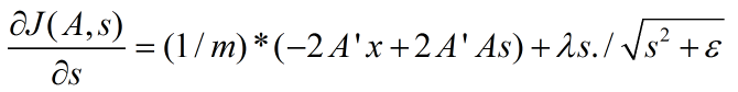
非拓扑结构下代价函数关于s的导数如下:
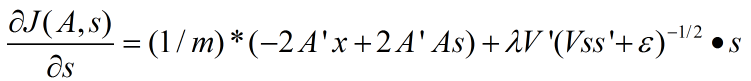
拓扑Sparse coding下代价函数关于s的导数为:
关于本程序的一点注释:
- 如果按照上面公式的和我们的理解,A是由学习到的基向量构成,S为每个样本在该基分解下的系数。在这里表示前提下,可以这样定义:A为n*k维,其中的每一列表示的是训练出来的基向量,S是k*m,其中的每一列是对应输入样本的sparse coding分解系数,当然了,此时的X是n*m了。即每一列表示的是一个样本数据。如果我们反过来表示(虽然这样理解不对,这里只是用不同的表示方法矩阵而已),即A表示输入数据X的分解系数(即编码值),而S是原始数据集训练出来的基的构成的,那么此时关于A,S,X三者的维度可以这样定义和解释:现假设有m个样本X,每个样本是个n维的向量,即X为m*n维的矩阵,需要用sparse coding学习k个特征,使得代价函数值最小,则其中的A是m*k维的,A中的第i行表示第i个样本分解后的系数值,S是k*n维的,S的第i行表示所学习到的第i个基。当然了,在本次实验和以后类似情况下我们还是用正确的版本,即第一种表示。
- 在matlab中,右除矩阵A和右乘inv(A)虽然在定义上式一样的,但是两者运行的结果有可能不同,右除的精度要高些。
- 注意拓扑结构下代价函数对s导数公式中的最后一项是点乘符号,也就是矩阵中对应元素的相乘,如果弄成了普通的矩阵乘法则就很难通过gradient checking了。
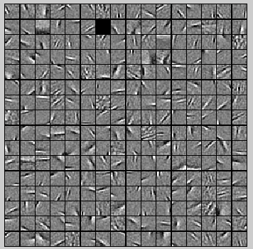
- 本程序训练样本IMAGE原图片尺寸512*512,共10张,从这10张大图片中提取2w张8*8的小patch图片,这些图片部分显示如下:

一些Matlab函数:
circshift:
该函数是将矩阵循环平移的函数,比如说B = circshift(A,shiftsize)是将矩阵A按照shiftsize的方式左右平移,一般hiftsize为一个多维的向量,第一个元素表示上下方向移动(更准确的说是在第一个维度上移动,这里只是考虑是2维矩阵的情况,后面的类似),如果为正表示向下移,第二个元素表示左右方向移动,如果向右表示向右移动。
rndperm:
该函数是随机产生一个行向量,比如randperm(n)产生一个n维的行向量,向量元素值为1~n,随机选取且不重复。而randperm(n,k)表示产生一个长为k的行向量,其元素也是在1到n之间,不能有重复。
questdlg:
button = questdlg('qstring','title','str1','str2','str3',default),这是一个对话框,对话框中的内容用qstring表示,标题为title,然后后面3个分别为对应yes,no,cancel按钮,最后的参数default为默认的对应按钮。
实验结果:
交叉优化参数中,给定s优化A时,由于A有直接的解析解,所以不需要通过lbfgs等优化算法求得,通过令代价函数对A的导函数为0,可以得到解析解为:
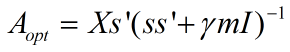
注意单位矩阵前一定要有个系数(即样本个数),不然在程序中直接用该方法求得的A是通过不了验证。
此时学习到的非拓扑结果为:
上面的结果有点难看,采用的是16*16大小的patch,而非8*8的。
采用cg优化,256个16*16大小的patch,其结果如下:
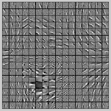
如果将patch改为8*8,121个特征点,结果如下(这个比较像样):

如果用lbfgs,256个16*16的,其结果如下(效果很差,说明优化方法对结果有影响):

实验部分代码及注释:
sparseCodeingExercise.m:
%% CS294A/CS294W Sparse Coding Exercise

%  Instructions
%  ------------
%
%  This file contains code that helps you get started on the
%  sparse coding exercise. In this exercise, you will need to modify
%  sparseCodingFeatureCost.m and sparseCodingWeightCost.m. You will also
%  need to modify this file, sparseCodingExercise.m slightly.

% Add the paths to your earlier exercises if necessary
% addpath /path/to/solution

%%======================================================================
%% STEP 0: Initialization
%  Here we initialize some parameters used for the exercise.

addpath minFunc;
numPatches = 20000;   % number of patches
numFeatures = 256;    % number of features to learn
patchDim = 16;         % patch dimension
visibleSize = patchDim * patchDim; %单通道灰度图,64维,学习121个特征

% dimension of the grouping region (poolDim x poolDim) for topographic sparse coding
poolDim = 3;

% number of patches per batch
batchNumPatches = 2000; %分成10个batch

lambda = 5e-5;  % L1-regularisation parameter (on features)
epsilon = 1e-5; % L1-regularisation epsilon |x| ~ sqrt(x^2 + epsilon)
gamma = 1e-2;   % L2-regularisation parameter (on basis)

%%======================================================================
%% STEP 1: Sample patches

images = load('IMAGES.mat');
images = images.IMAGES;
patches = sampleIMAGES(images, patchDim, numPatches);
display_network(patches(:, 1:64));

%%======================================================================
%% STEP 3: Iterative optimization
%  Once you have implemented the cost functions, you can now optimize for
%  the objective iteratively. The code to do the iterative optimization
%  using mini-batching and good initialization of the features has already
%  been included for you.
%
%  However, you will still need to derive and fill in the analytic solution
%  for optimizing the weight matrix given the features.
%  Derive the solution and implement it in the code below, verify the
%  gradient as described in the instructions below, and then run the
%  iterative optimization.

% Initialize options for minFunc
options.Method = 'cg';
options.display = 'off';
options.verbose = 0;

% Initialize matrices
weightMatrix = rand(visibleSize, numFeatures);%64*121
featureMatrix = rand(numFeatures, batchNumPatches);%121*2000

% Initialize grouping matrix
assert(floor(sqrt(numFeatures)) ^2 == numFeatures, 'numFeatures should be a perfect square');
donutDim = floor(sqrt(numFeatures));
assert(donutDim * donutDim == numFeatures,'donutDim^2 must be equal to numFeatures');

groupMatrix = zeros(numFeatures, donutDim, donutDim);%121*11*11
groupNum = 1;
for row = 1:donutDim
    for col = 1:donutDim
        groupMatrix(groupNum, 1:poolDim, 1:poolDim) = 1;%poolDim=3
        groupNum = groupNum + 1;
        groupMatrix = circshift(groupMatrix, [0 0 -1]);
    end
    groupMatrix = circshift(groupMatrix, [0 -1, 0]);
end
groupMatrix = reshape(groupMatrix, numFeatures, numFeatures);%121*121

if isequal(questdlg('Initialize grouping matrix for topographic or non-topographic sparse coding?', 'Topographic/non-topographic?', 'Non-topographic', 'Topographic', 'Non-topographic'), 'Non-topographic')
    groupMatrix = eye(numFeatures);%非拓扑结构时的groupMatrix矩阵
end

% Initial batch
indices = randperm(numPatches);%1*20000
indices = indices(1:batchNumPatches);%1*2000
batchPatches = patches(:, indices);

fprintf('%6s%12s%12s%12s%12s\n','Iter', 'fObj','fResidue','fSparsity','fWeight');
warning off;
for iteration = 1:200
  %  iteration = 1;
    error = weightMatrix * featureMatrix - batchPatches;
    error = sum(error(:) .^ 2) / batchNumPatches;  %说明重构误差需要考虑样本数
    fResidue = error;
    num_batches = size(batchPatches,2);
    R = groupMatrix * (featureMatrix .^ 2);
    R = sqrt(R + epsilon);
    fSparsity = lambda * sum(R(:));    %稀疏项和权值惩罚项不需要考虑样本数

    fWeight = gamma * sum(weightMatrix(:) .^ 2);

    %上面的那些权值都是随机初始化的
    fprintf('  %4d  %10.4f  %10.4f  %10.4f  %10.4f\n', iteration, fResidue+fSparsity+fWeight, fResidue, fSparsity, fWeight)

    % Select a new batch
    indices = randperm(numPatches);
    indices = indices(1:batchNumPatches);
    batchPatches = patches(:, indices);

    % Reinitialize featureMatrix with respect to the new
    % 对featureMatrix重新初始化,按照网页教程上介绍的方法进行
    featureMatrix = weightMatrix' * batchPatches;
    normWM = sum(weightMatrix .^ 2)';
    featureMatrix = bsxfun(@rdivide, featureMatrix, normWM);

    % Optimize for feature matrix
    options.maxIter = 20;
    %给定权值初始值,优化特征值矩阵
    [featureMatrix, cost] = minFunc( @(x) sparseCodingFeatureCost(weightMatrix, x, visibleSize, numFeatures, batchPatches, gamma, lambda, epsilon, groupMatrix), ...
                                           featureMatrix(:), options);
    featureMatrix = reshape(featureMatrix, numFeatures, batchNumPatches);
    weightMatrix = (batchPatches*featureMatrix')/(gamma*num_batches*eye(size(featureMatrix,1))+featureMatrix*featureMatrix');
    [cost, grad] = sparseCodingWeightCost(weightMatrix, featureMatrix, visibleSize, numFeatures, batchPatches, gamma, lambda, epsilon, groupMatrix);

end
    figure;
    display_network(weightMatrix);
sparseCodingWeightCost.m:
function [cost, grad] = sparseCodingWeightCost(weightMatrix, featureMatrix, visibleSize, numFeatures,  patches, gamma, lambda, epsilon, groupMatrix)
%sparseCodingWeightCost - given the features in featureMatrix,
%                         computes the cost and gradient with respect to
%                         the weights, given in weightMatrix
% parameters
%   weightMatrix  - the weight matrix. weightMatrix(:, c) is the cth basis
%                   vector.
%   featureMatrix - the feature matrix. featureMatrix(:, c) is the features
%                   for the cth example
%   visibleSize   - number of pixels in the patches
%   numFeatures   - number of features
%   patches       - patches
%   gamma         - weight decay parameter (on weightMatrix)
%   lambda        - L1 sparsity weight (on featureMatrix)
%   epsilon       - L1 sparsity epsilon
%   groupMatrix   - the grouping matrix. groupMatrix(r, :) indicates the
%                   features included in the rth group. groupMatrix(r, c)
%                   is 1 if the cth feature is in the rth group and 0
%                   otherwise.

    if exist('groupMatrix', 'var')
        assert(size(groupMatrix, 2) == numFeatures, 'groupMatrix has bad dimension');
    else
        groupMatrix = eye(numFeatures);%非拓扑的sparse coding中,相当于groupMatrix为单位对角矩阵
    end

    numExamples = size(patches, 2);%测试代码时为5

    weightMatrix = reshape(weightMatrix, visibleSize, numFeatures);%其实传入进来的就是这些东西
    featureMatrix = reshape(featureMatrix, numFeatures, numExamples);

    % -------------------- YOUR CODE HERE --------------------
    % Instructions:
    %   Write code to compute the cost and gradient with respect to the
    %   weights given in weightMatrix.
    % -------------------- YOUR CODE HERE --------------------
    %% 求目标的代价函数
    delta = weightMatrix*featureMatrix-patches;
    fResidue = sum(sum(delta.^2))./numExamples;%重构误差
    fWeight = gamma*sum(sum(weightMatrix.^2));%防止基内元素值过大
%     sparsityMatrix = sqrt(groupMatrix*(featureMatrix.^2)+epsilon);
%     fSparsity = lambda*sum(sparsityMatrix(:)); %对特征系数性的惩罚值
%     cost = fResidue+fWeight+fSparsity; %目标的代价函数
    cost = fResidue+fWeight;

    %% 求目标代价函数的偏导函数
    grad = (2*weightMatrix*featureMatrix*featureMatrix'-2*patches*featureMatrix')./numExamples+2*gamma*weightMatrix;
    grad = grad(:);

end
sparseCodingFeatureCost .m:
function [cost, grad] = sparseCodingFeatureCost(weightMatrix, featureMatrix, visibleSize, numFeatures, patches, gamma, lambda, epsilon, groupMatrix)
%sparseCodingFeatureCost - given the weights in weightMatrix,
%                          computes the cost and gradient with respect to
%                          the features, given in featureMatrix
% parameters
%   weightMatrix  - the weight matrix. weightMatrix(:, c) is the cth basis
%                   vector.
%   featureMatrix - the feature matrix. featureMatrix(:, c) is the features
%                   for the cth example
%   visibleSize   - number of pixels in the patches
%   numFeatures   - number of features
%   patches       - patches
%   gamma         - weight decay parameter (on weightMatrix)
%   lambda        - L1 sparsity weight (on featureMatrix)
%   epsilon       - L1 sparsity epsilon
%   groupMatrix   - the grouping matrix. groupMatrix(r, :) indicates the
%                   features included in the rth group. groupMatrix(r, c)
%                   is 1 if the cth feature is in the rth group and 0
%                   otherwise.

    isTopo = 1;
%     L = size(groupMatrix,1);
%     [K M] = size(featureMatrix);
    if exist('groupMatrix', 'var')
        assert(size(groupMatrix, 2) == numFeatures, 'groupMatrix has bad dimension');
        if(isequal(groupMatrix,eye(numFeatures)));
            isTopo = 0;
        end
    else
        groupMatrix = eye(numFeatures);
         isTopo = 0;
    end

    numExamples = size(patches, 2);
    weightMatrix = reshape(weightMatrix, visibleSize, numFeatures);
    featureMatrix = reshape(featureMatrix, numFeatures, numExamples);

    % -------------------- YOUR CODE HERE --------------------
    % Instructions:
    %   Write code to compute the cost and gradient with respect to the
    %   features given in featureMatrix.
    %   You may wish to write the non-topographic version, ignoring
    %   the grouping matrix groupMatrix first, and extend the
    %   non-topographic version to the topographic version later.
    % -------------------- YOUR CODE HERE --------------------


    %% 求目标的代价函数
    delta = weightMatrix*featureMatrix-patches;
    fResidue = sum(sum(delta.^2))./numExamples;%重构误差
%     fWeight = gamma*sum(sum(weightMatrix.^2));%防止基内元素值过大
    sparsityMatrix = sqrt(groupMatrix*(featureMatrix.^2)+epsilon);
    fSparsity = lambda*sum(sparsityMatrix(:)); %对特征系数性的惩罚值
%     cost = fResidue++fSparsity+fWeight;%此时A为常量,可以不用
    cost = fResidue++fSparsity;

    %% 求目标代价函数的偏导函数
    gradResidue = (-2*weightMatrix'*patches+2*weightMatrix'*weightMatrix*featureMatrix)./numExamples;

    % 非拓扑结构时:
    if ~isTopo
        gradSparsity = lambda*(featureMatrix./sparsityMatrix);
    end

    % 拓扑结构时
    if isTopo
%         gradSparsity = lambda*groupMatrix'*(groupMatrix*(featureMatrix.^2)+epsilon).^(-0.5).*featureMatrix;%一定要小心最后一项是内积乘法
        gradSparsity = lambda*groupMatrix'*(groupMatrix*(featureMatrix.^2)+epsilon).^(-0.5).*featureMatrix;%一定要小心最后一项是内积乘法
    end
    grad = gradResidue+gradSparsity;
    grad = grad(:);

end
sampleIMAGES.m:
function patches = sampleIMAGES(images, patchsize,numpatches)
% sampleIMAGES
% Returns 10000 patches for training

% load IMAGES;    % load images from disk

%patchsize = 8;  % we'll use 8x8 patches
%numpatches = 10000;

% Initialize patches with zeros.  Your code will fill in this matrix--one
% column per patch, 10000 columns.
patches = zeros(patchsize*patchsize, numpatches);

%% ---------- YOUR CODE HERE --------------------------------------
%  Instructions: Fill in the variable called "patches" using data
%  from IMAGES.
%
%  IMAGES is a 3D array containing 10 images
%  For instance, IMAGES(:,:,6) is a 512x512 array containing the 6th image,
%  and you can type "imagesc(IMAGES(:,:,6)), colormap gray;" to visualize
%  it. (The contrast on these images look a bit off because they have
%  been preprocessed using using "whitening."  See the lecture notes for
%  more details.) As a second example, IMAGES(21:30,21:30,1) is an image
%  patch corresponding to the pixels in the block (21,21) to (30,30) of
%  Image 1
for imageNum = 1:10%在每张图片中随机选取1000个patch,共10000个patch
    [rowNum colNum] = size(images(:,:,imageNum));
    for patchNum = 1:2000%实现每张图片选取1000个patch
        xPos = randi([1,rowNum-patchsize+1]);
        yPos = randi([1, colNum-patchsize+1]);
        patches(:,(imageNum-1)*2000+patchNum) = reshape(images(xPos:xPos+patchsize-1,yPos:yPos+patchsize-1,...
                                                        imageNum),patchsize*patchsize,1);
    end
end


%% ---------------------------------------------------------------
% For the autoencoder to work well we need to normalize the data
% Specifically, since the output of the network is bounded between [0,1]
% (due to the sigmoid activation function), we have to make sure
% the range of pixel values is also bounded between [0,1]
% patches = normalizeData(patches);

end


%% ---------------------------------------------------------------
function patches = normalizeData(patches)

% Squash data to [0.1, 0.9] since we use sigmoid as the activation
% function in the output layer

% Remove DC (mean of images).
patches = bsxfun(@minus, patches, mean(patches));

% Truncate to +/-3 standard deviations and scale to -1 to 1
pstd = 3 * std(patches(:));
patches = max(min(patches, pstd), -pstd) / pstd;%因为根据3sigma法则,95%以上的数据都在该区域内
                                                % 这里转换后将数据变到了-1到1之间

% Rescale from [-1,1] to [0.1,0.9]
patches = (patches + 1) * 0.4 + 0.1;

end
实验总结:
拓扑结构的Sparse coding未完成,跑出来没有效果,还望有人指导下。
2013.5.6:
已解决非拓扑下的Sparse coding,那时候出现的问题是因为在代价函数中,重构误差那一项没有除样本数(下面博文回复中网友给的提示),导致代价函数,导数,以及A的解析解都相应错了。
但是拓扑Sparse Coding依旧没有训练出来,因为训练过程中代价函数的值不是递减的,而是基本无规律。
2013.5.14:
基本解决了拓扑下的Sparse coding。以前训练不出特征来主要原因是在sampleIMAGES.m里没有将最后的patches归一化注释掉(个人猜测:采样前的大图片是经过白化了的,所以如果后面继续用那个带误差的归一化,可能引入更大的误差,导致给定的样本不适合Sparse coding),另外就是根据群里网友@地皮菜的提示,将优化算法由lbfgs改为cg就可以得出像样的结果。由此可见,不同的优化算法对最终的结果也是有影响的。
参考资料:
Deep learning:二十六(Sparse coding简单理解)
Deep learning:二十七(Sparse coding中关于矩阵的范数求导)
Deep learning:二十八(使用BP算法思想求解Sparse coding中矩阵范数导数)

