

Deep learning:二十四(stacked autoencoder练习)
前言:
本次是练习2个隐含层的网络的训练方法,每个网络层都是用的sparse autoencoder思想,利用两个隐含层的网络来提取出输入数据的特征。本次实验验要完成的任务是对MINST进行手写数字识别,实验内容及步骤参考网页教程Exercise: Implement deep networks for digit classification。当提取出手写数字图片的特征后,就用softmax进行对其进行分类。关于MINST的介绍可以参考网页:MNIST Dataset。本文的理论介绍也可以参考前面的博文:Deep learning:十六(deep networks)。
实验基础:
进行deep network的训练方法大致如下:
1. 用原始输入数据作为输入,训练出(利用sparse autoencoder方法)第一个隐含层结构的网络参数,并将用训练好的参数算出第1个隐含层的输出。
2. 把步骤1的输出作为第2个网络的输入,用同样的方法训练第2个隐含层网络的参数。
3. 用步骤2 的输出作为多分类器softmax的输入,然后利用原始数据的标签来训练出softmax分类器的网络参数。
4. 计算2个隐含层加softmax分类器整个网络一起的损失函数,以及整个网络对每个参数的偏导函数值。
5. 用步骤1,2和3的网络参数作为整个深度网络(2个隐含层,1个softmax输出层)参数初始化的值,然后用lbfs算法迭代求出上面损失函数最小值附近处的参数值,并作为整个网络最后的最优参数值。
上面的训练过程是针对使用softmax分类器进行的,而softmax分类器的损失函数等是有公式进行计算的。所以在进行参数校正时,可以对把所有网络看做是一个整体,然后计算整个网络的损失函数和其偏导,这样的话当我们有了标注好了的数据后,就可以用前面训练好了的参数作为初始参数,然后用优化算法求得整个网络的参数了。但如果我们后面的分类器不是用的softmax分类器,而是用的其它的,比如svm,随机森林等,这个时候前面特征提取的网络参数已经预训练好了,用该参数是可以初始化前面的网络,但是此时该怎么微调呢?因为此时标注的数值只能在后面的分类器中才用得到,所以没法计算系统的损失函数等。难道又要将前面n层网络的最终输出等价于第一层网络的输入(也就是多网络的sparse autoencoder)?本人暂时还没弄清楚,日后应该会想明白的。
关于深度网络的学习几个需要注意的小点(假设隐含层为2层):
- 利用sparse autoencoder进行预训练时,需要依次计算出每个隐含层的输出,如果后面是采用softmax分类器的话,则同样也需要用最后一个隐含层的输出作为softmax的输入来训练softmax的网络参数。
- 由步骤1可知,在进行参数校正之前是需要对分类器的参数进行预训练的。且在进行参数校正(Finetuning )时是将所有的隐含层看做是一个单一的网络层,因此每一次迭代就可以更新所有网络层的参数。
另外在实际的训练过程中可以看到,训练第一个隐含层所用的时间较长,应该需要训练的参数矩阵为200*784(没包括b参数),训练第二个隐含层的时间较第一个隐含层要短些,主要原因是此时只需学习到200*200的参数矩阵,其参数个数大大减小。而训练softmax的时间更短,那是因为它的参数个数更少,且损失函数和偏导的计算公式也没有前面两层的复杂。最后对整个网络的微调所用的时间和第二个隐含层的训练时间长短差不多。
程序中部分函数:
[params, netconfig] = stack2params(stack)
是将stack层次的网络参数(可能是多个参数)转换成一个向量params,这样有利用使用各种优化算法来进行优化操作。Netconfig中保存的是该网络的相关信息,其中netconfig.inputsize表示的是网络的输入层节点的个数。netconfig.layersizes中的元素分别表示每一个隐含层对应节点的个数。
[ cost, grad ] = stackedAECost(theta, inputSize, hiddenSize, numClasses, netconfig,lambda, data, labels)
该函数内部实现整个网络损失函数和损失函数对每个参数偏导的计算。其中损失函数是个实数值,当然就只有1个了,其计算方法是根据sofmax分类器来计算的,只需知道标签值和softmax输出层的值即可。而损失函数对所有参数的偏导却有很多个,因此每个参数处应该就有一个偏导值,这些参数不仅包括了多个隐含层的,而且还包括了softmax那个网络层的。其中softmax那部分的偏导是根据其公式直接获得,而深度网络层那部分这通过BP算法方向推理得到(即先计算每一层的误差值,然后利用该误差值计算参数w和b)。
stack = params2stack(params, netconfig)
和上面的函数功能相反,是吧一个向量参数按照深度网络的结构依次展开。
[pred] = stackedAEPredict(theta, inputSize, hiddenSize, numClasses, netconfig, data)
这个函数其实就是对输入的data数据进行预测,看该data对应的输出类别是多少。其中theta为整个网络的参数(包括了分类器部分的网络),numClasses为所需分类的类别,netconfig为网络的结构参数。
[h, array] = display_network(A, opt_normalize, opt_graycolor, cols, opt_colmajor)
该函数是用来显示矩阵A的,此时要求A中的每一列为一个权值,并且A是完全平方数。函数运行后会将A中每一列显示为一个小的patch图像,具体的有多少个patch和patch之间该怎么摆设是程序内部自动决定的。
matlab内嵌函数:
struct:
s = sturct;表示创建一个结构数组s。
nargout:
表示函数输出参数的个数。
save:
比如函数save('saves/step2.mat', 'sae1OptTheta');则要求当前目录下有saves这个目录,否则该语句会调用失败的。
实验结果:
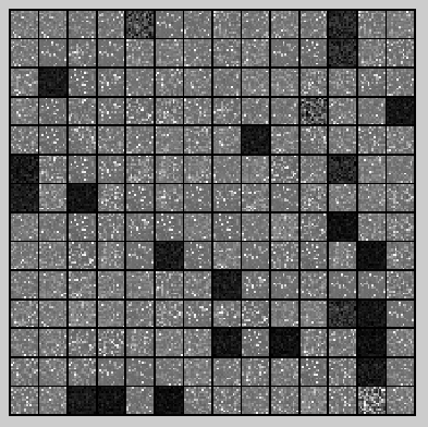
第一个隐含层的特征值如下所示:

第二个隐含层的特征值显示不知道该怎么弄,因为第二个隐含层每个节点都是对应的200维,用display_network这个函数去显示的话是不行的,它只能显示维数能够开平方的那些特征,所以不知道是该将200弄成20*10,还是弄成16*25好,很好奇关于deep learning那么多文章中第二层网络是怎么显示的,将200分解后的显示哪个具有代表性呢?待定。所以这里暂且不显示,因为截取200前面的196位用display_network来显示的话,什么都看不出来:
没有经过网络参数微调时的识别准去率为:
Before Finetuning Test Accuracy: 92.190%
经过了网络参数微调后的识别准确率为:
After Finetuning Test Accuracy: 97.670%
实验主要部分代码及注释:
stackedAEExercise.m:
%% CS294A/CS294W Stacked Autoencoder Exercise

%  Instructions
%  ------------
%
%  This file contains code that helps you get started on the
%  sstacked autoencoder exercise. You will need to complete code in
%  stackedAECost.m
%  You will also need to have implemented sparseAutoencoderCost.m and
%  softmaxCost.m from previous exercises. You will need the initializeParameters.m
%  loadMNISTImages.m, and loadMNISTLabels.m files from previous exercises.
%
%  For the purpose of completing the assignment, you do not need to
%  change the code in this file.
%
%%======================================================================
%% STEP 0: Here we provide the relevant parameters values that will
%  allow your sparse autoencoder to get good filters; you do not need to
%  change the parameters below.

DISPLAY = true;
inputSize = 28 * 28;
numClasses = 10;
hiddenSizeL1 = 200;    % Layer 1 Hidden Size
hiddenSizeL2 = 200;    % Layer 2 Hidden Size
sparsityParam = 0.1;   % desired average activation of the hidden units.
                       % (This was denoted by the Greek alphabet rho, which looks like a lower-case "p",
                       %  in the lecture notes).
lambda = 3e-3;         % weight decay parameter
beta = 3;              % weight of sparsity penalty term

%%======================================================================
%% STEP 1: Load data from the MNIST database
%
%  This loads our training data from the MNIST database files.

% Load MNIST database files
trainData = loadMNISTImages('train-images.idx3-ubyte');
trainLabels = loadMNISTLabels('train-labels.idx1-ubyte');

trainLabels(trainLabels == 0) = 10; % Remap 0 to 10 since our labels need to start from 1

%%======================================================================
%% STEP 2: Train the first sparse autoencoder
%  This trains the first sparse autoencoder on the unlabelled STL training
%  images.
%  If you've correctly implemented sparseAutoencoderCost.m, you don't need
%  to change anything here.
%  Randomly initialize the parameters
sae1Theta = initializeParameters(hiddenSizeL1, inputSize);

%% ---------------------- YOUR CODE HERE  ---------------------------------
%  Instructions: Train the first layer sparse autoencoder, this layer has
%                an hidden size of "hiddenSizeL1"
%                You should store the optimal parameters in sae1OptTheta
addpath minFunc/;
options = struct;
options.Method = 'lbfgs';
options.maxIter = 400;
options.display = 'on';
[sae1OptTheta, cost] =  minFunc(@(p)sparseAutoencoderCost(p,...
    inputSize,hiddenSizeL1,lambda,sparsityParam,beta,trainData),sae1Theta,options);%训练出第一层网络的参数
save('saves/step2.mat', 'sae1OptTheta');

if DISPLAY
  W1 = reshape(sae1OptTheta(1:hiddenSizeL1 * inputSize), hiddenSizeL1, inputSize);
  display_network(W1');
end
% -------------------------------------------------------------------------

%%======================================================================
%% STEP 2: Train the second sparse autoencoder
%  This trains the second sparse autoencoder on the first autoencoder
%  featurse.
%  If you've correctly implemented sparseAutoencoderCost.m, you don't need
%  to change anything here.

[sae1Features] = feedForwardAutoencoder(sae1OptTheta, hiddenSizeL1, ...
                                        inputSize, trainData);

%  Randomly initialize the parameters
sae2Theta = initializeParameters(hiddenSizeL2, hiddenSizeL1);

%% ---------------------- YOUR CODE HERE  ---------------------------------
%  Instructions: Train the second layer sparse autoencoder, this layer has
%                an hidden size of "hiddenSizeL2" and an inputsize of
%                "hiddenSizeL1"
%
%                You should store the optimal parameters in sae2OptTheta

[sae2OptTheta, cost] =  minFunc(@(p)sparseAutoencoderCost(p,...
    hiddenSizeL1,hiddenSizeL2,lambda,sparsityParam,beta,sae1Features),sae2Theta,options);%训练出第一层网络的参数
save('saves/step3.mat', 'sae2OptTheta');

figure;
if DISPLAY
  W11 = reshape(sae1OptTheta(1:hiddenSizeL1 * inputSize), hiddenSizeL1, inputSize);
  W12 = reshape(sae2OptTheta(1:hiddenSizeL2 * hiddenSizeL1), hiddenSizeL2, hiddenSizeL1);
  % TODO(zellyn): figure out how to display a 2-level network
%  display_network(log(W11' ./ (1-W11')) * W12');
%   W12_temp = W12(1:196,1:196);
%   display_network(W12_temp');
%   figure;
%   display_network(W12_temp');
end
% -------------------------------------------------------------------------

%%======================================================================
%% STEP 3: Train the softmax classifier
%  This trains the sparse autoencoder on the second autoencoder features.
%  If you've correctly implemented softmaxCost.m, you don't need
%  to change anything here.

[sae2Features] = feedForwardAutoencoder(sae2OptTheta, hiddenSizeL2, ...
                                        hiddenSizeL1, sae1Features);

%  Randomly initialize the parameters
saeSoftmaxTheta = 0.005 * randn(hiddenSizeL2 * numClasses, 1);


%% ---------------------- YOUR CODE HERE  ---------------------------------
%  Instructions: Train the softmax classifier, the classifier takes in
%                input of dimension "hiddenSizeL2" corresponding to the
%                hidden layer size of the 2nd layer.
%
%                You should store the optimal parameters in saeSoftmaxOptTheta
%
%  NOTE: If you used softmaxTrain to complete this part of the exercise,
%        set saeSoftmaxOptTheta = softmaxModel.optTheta(:);


softmaxLambda = 1e-4;
numClasses = 10;
softoptions = struct;
softoptions.maxIter = 400;
softmaxModel = softmaxTrain(hiddenSizeL2,numClasses,softmaxLambda,...
                            sae2Features,trainLabels,softoptions);
saeSoftmaxOptTheta = softmaxModel.optTheta(:);

save('saves/step4.mat', 'saeSoftmaxOptTheta');
% -------------------------------------------------------------------------

%%======================================================================
%% STEP 5: Finetune softmax model

% Implement the stackedAECost to give the combined cost of the whole model
% then run this cell.

% Initialize the stack using the parameters learned
stack = cell(2,1);
%其中的saelOptTheta和sae1ptTheta都是包含了sparse autoencoder的重建层网络权值的
stack{1}.w = reshape(sae1OptTheta(1:hiddenSizeL1*inputSize), ...
                     hiddenSizeL1, inputSize);
stack{1}.b = sae1OptTheta(2*hiddenSizeL1*inputSize+1:2*hiddenSizeL1*inputSize+hiddenSizeL1);
stack{2}.w = reshape(sae2OptTheta(1:hiddenSizeL2*hiddenSizeL1), ...
                     hiddenSizeL2, hiddenSizeL1);
stack{2}.b = sae2OptTheta(2*hiddenSizeL2*hiddenSizeL1+1:2*hiddenSizeL2*hiddenSizeL1+hiddenSizeL2);

% Initialize the parameters for the deep model
[stackparams, netconfig] = stack2params(stack);
stackedAETheta = [ saeSoftmaxOptTheta ; stackparams ];%stackedAETheta是个向量,为整个网络的参数,包括分类器那部分,且分类器那部分的参数放前面

%% ---------------------- YOUR CODE HERE  ---------------------------------
%  Instructions: Train the deep network, hidden size here refers to the '
%                dimension of the input to the classifier, which corresponds
%                to "hiddenSizeL2".
%
%

[stackedAEOptTheta, cost] =  minFunc(@(p)stackedAECost(p,inputSize,hiddenSizeL2,...
                         numClasses, netconfig,lambda, trainData, trainLabels),...
                        stackedAETheta,options);%训练出第一层网络的参数
save('saves/step5.mat', 'stackedAEOptTheta');

figure;
if DISPLAY
  optStack = params2stack(stackedAEOptTheta(hiddenSizeL2*numClasses+1:end), netconfig);
  W11 = optStack{1}.w;
  W12 = optStack{2}.w;
  % TODO(zellyn): figure out how to display a 2-level network
  % display_network(log(1 ./ (1-W11')) * W12');
end
% -------------------------------------------------------------------------

%%======================================================================
%% STEP 6: Test
%  Instructions: You will need to complete the code in stackedAEPredict.m
%                before running this part of the code
%

% Get labelled test images
% Note that we apply the same kind of preprocessing as the training set
testData = loadMNISTImages('t10k-images.idx3-ubyte');
testLabels = loadMNISTLabels('t10k-labels.idx1-ubyte');

testLabels(testLabels == 0) = 10; % Remap 0 to 10

[pred] = stackedAEPredict(stackedAETheta, inputSize, hiddenSizeL2, ...
                          numClasses, netconfig, testData);

acc = mean(testLabels(:) == pred(:));
fprintf('Before Finetuning Test Accuracy: %0.3f%%\n', acc * 100);

[pred] = stackedAEPredict(stackedAEOptTheta, inputSize, hiddenSizeL2, ...
                          numClasses, netconfig, testData);

acc = mean(testLabels(:) == pred(:));
fprintf('After Finetuning Test Accuracy: %0.3f%%\n', acc * 100);

% Accuracy is the proportion of correctly classified images
% The results for our implementation were:
%
% Before Finetuning Test Accuracy: 87.7%
% After Finetuning Test Accuracy:  97.6%
%
% If your values are too low (accuracy less than 95%), you should check
% your code for errors, and make sure you are training on the
% entire data set of 60000 28x28 training images
% (unless you modified the loading code, this should be the case)
stackedAECost.m:
function [ cost, grad ] = stackedAECost(theta, inputSize, hiddenSize, ...
                                              numClasses, netconfig, ...
                                              lambda, data, labels)

% stackedAECost: Takes a trained softmaxTheta and a training data set with labels,
% and returns cost and gradient using a stacked autoencoder model. Used for
% finetuning.

% theta: trained weights from the autoencoder
% visibleSize: the number of input units
% hiddenSize:  the number of hidden units *at the 2nd layer*
% numClasses:  the number of categories
% netconfig:   the network configuration of the stack
% lambda:      the weight regularization penalty
% data: Our matrix containing the training data as columns.  So, data(:,i) is the i-th training example.
% labels: A vector containing labels, where labels(i) is the label for the
% i-th training example


%% Unroll softmaxTheta parameter

% We first extract the part which compute the softmax gradient
softmaxTheta = reshape(theta(1:hiddenSize*numClasses), numClasses, hiddenSize);

% Extract out the "stack"
stack = params2stack(theta(hiddenSize*numClasses+1:end), netconfig);

% You will need to compute the following gradients
softmaxThetaGrad = zeros(size(softmaxTheta));
stackgrad = cell(size(stack));
for d = 1:numel(stack)
    stackgrad{d}.w = zeros(size(stack{d}.w));
    stackgrad{d}.b = zeros(size(stack{d}.b));
end

cost = 0; % You need to compute this

% You might find these variables useful
M = size(data, 2);
groundTruth = full(sparse(labels, 1:M, 1));


%% --------------------------- YOUR CODE HERE -----------------------------
%  Instructions: Compute the cost function and gradient vector for
%                the stacked autoencoder.
%
%                You are given a stack variable which is a cell-array of
%                the weights and biases for every layer. In particular, you
%                can refer to the weights of Layer d, using stack{d}.w and
%                the biases using stack{d}.b . To get the total number of
%                layers, you can use numel(stack).
%
%                The last layer of the network is connected to the softmax
%                classification layer, softmaxTheta.
%
%                You should compute the gradients for the softmaxTheta,
%                storing that in softmaxThetaGrad. Similarly, you should
%                compute the gradients for each layer in the stack, storing
%                the gradients in stackgrad{d}.w and stackgrad{d}.b
%                Note that the size of the matrices in stackgrad should
%                match exactly that of the size of the matrices in stack.
%

depth = numel(stack);
z = cell(depth+1,1);
a = cell(depth+1, 1);
a{1} = data;

for layer = (1:depth)
  z{layer+1} = stack{layer}.w * a{layer} + repmat(stack{layer}.b, [1, size(a{layer},2)]);
  a{layer+1} = sigmoid(z{layer+1});
end

M = softmaxTheta * a{depth+1};
M = bsxfun(@minus, M, max(M));
p = bsxfun(@rdivide, exp(M), sum(exp(M)));

cost = -1/numClasses * groundTruth(:)' * log(p(:)) + lambda/2 * sum(softmaxTheta(:) .^ 2);
softmaxThetaGrad = -1/numClasses * (groundTruth - p) * a{depth+1}' + lambda * softmaxTheta;

d = cell(depth+1);

d{depth+1} = -(softmaxTheta' * (groundTruth - p)) .* a{depth+1} .* (1-a{depth+1});

for layer = (depth:-1:2)
  d{layer} = (stack{layer}.w' * d{layer+1}) .* a{layer} .* (1-a{layer});
end

for layer = (depth:-1:1)
  stackgrad{layer}.w = (1/numClasses) * d{layer+1} * a{layer}';
  stackgrad{layer}.b = (1/numClasses) * sum(d{layer+1}, 2);
end

% -------------------------------------------------------------------------

%% Roll gradient vector
grad = [softmaxThetaGrad(:) ; stack2params(stackgrad)];

end


% You might find this useful
function sigm = sigmoid(x)
    sigm = 1 ./ (1 + exp(-x));
end
stackedAEPredict.m:
function [pred] = stackedAEPredict(theta, inputSize, hiddenSize, numClasses, netconfig, data) % stackedAEPredict: Takes a trained theta and a test data set, % and returns the predicted labels for each example. % theta: trained weights from the autoencoder % visibleSize: the number of input units % hiddenSize: the number of hidden units *at the 2nd layer* % numClasses: the number of categories % data: Our matrix containing the training data as columns. So, data(:,i) is the i-th training example. % Your code should produce the prediction matrix % pred, where pred(i) is argmax_c P(y(c) | x(i)). %% Unroll theta parameter % We first extract the part which compute the softmax gradient softmaxTheta = reshape(theta(1:hiddenSize*numClasses), numClasses, hiddenSize); % Extract out the "stack" stack = params2stack(theta(hiddenSize*numClasses+1:end), netconfig); %% ---------- YOUR CODE HERE -------------------------------------- % Instructions: Compute pred using theta assuming that the labels start % from 1. depth = numel(stack); z = cell(depth+1,1); a = cell(depth+1, 1); a{1} = data; for layer = (1:depth) z{layer+1} = stack{layer}.w * a{layer} + repmat(stack{layer}.b, [1, size(a{layer},2)]); a{layer+1} = sigmoid(z{layer+1}); end [~, pred] = max(softmaxTheta * a{depth+1});%閫夋鐜囨渶澶х殑閭d釜杈撳嚭鍊� % ----------------------------------------------------------- end % You might find this useful function sigm = sigmoid(x) sigm = 1 ./ (1 + exp(-x)); end
参考资料:
Exercise: Implement deep networks for digit classification
Deep learning:十六(deep networks)

