
神经网络量化入门--Folding BN ReLU代码实现
本文首发于公众号
上一篇文章介绍了如何把 BatchNorm 和 ReLU 合并到 Conv 中,这篇文章会介绍具体的代码实现。本文相关代码都可以在 github 上找到。
Folding BN
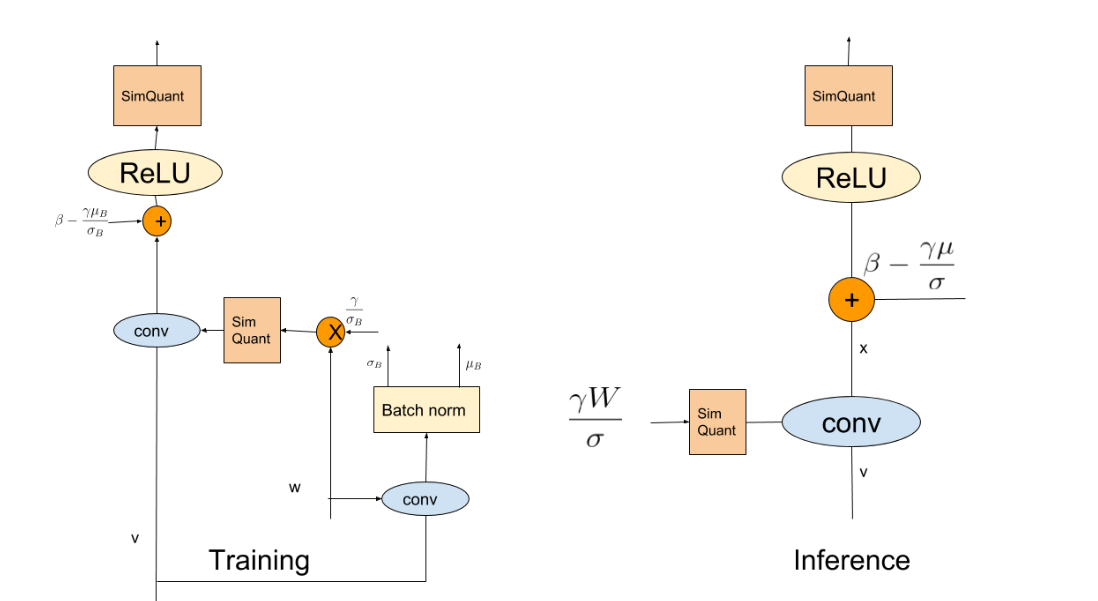
回顾一下前文把 BN 合并到 Conv 中的公式:
其中,\(x\) 是卷积层的输入,\(w\)、\(b\) 分别是 Conv 的参数 weight 和 bias,\(\gamma\)、\(\beta\) 是 BN 层的参数。
对于 BN 的合并,首先,我们需要熟悉 pytorch 中的 BatchNorm2d 模块。
pytorch 中的BatchNorm2d针对 feature map 的每一个 channel 都会计算一个均值和方差,所以公式 (1) 需要对 weight 和 bias 进行 channel wise 的计算。另外,BatchNorm2d中有一个布尔变量 affine,当该变量为 true 的时候,(1) 式中的 \(\gamma\) 和 \(\beta\) 就是可学习的, BatchNorm2d会中有两个变量:weight和bias,来分别存放这两个参数。而当affine为 false 的时候,就直接默认 \(\gamma=1\),\(\beta=0\),相当于 BN 中没有可学习的参数。默认情况下,我们都设置 affine=True。
我们沿用之前的代码,先定义一个 QConvBNReLU 模块:
class QConvBNReLU(QModule):

    def __init__(self, conv_module, bn_module, qi=True, qo=True, num_bits=8):
        super(QConvBNReLU, self).__init__(qi=qi, qo=qo, num_bits=num_bits)
        self.num_bits = num_bits
        self.conv_module = conv_module
        self.bn_module = bn_module
        self.qw = QParam(num_bits=num_bits)
这个模块会把全精度网络中的 Conv2d 和 BN 接收进来,并重新封装成量化的模块。
接着,定义合并 BN 后的 forward 流程:
    def forward(self, x):

        if hasattr(self, 'qi'):
            self.qi.update(x)
            x = FakeQuantize.apply(x, self.qi)

        if self.training: # 开启BN层训练
            y = F.conv2d(x, self.conv_module.weight, self.conv_module.bias,
                            stride=self.conv_module.stride,
                            padding=self.conv_module.padding,
                            dilation=self.conv_module.dilation,
                            groups=self.conv_module.groups)
            y = y.permute(1, 0, 2, 3) # NCHW -> CNHW
            y = y.contiguous().view(self.conv_module.out_channels, -1) # CNHW -> (C,NHW),这一步是为了方便channel wise计算均值和方差
            mean = y.mean(1)
            var = y.var(1)
            self.bn_module.running_mean = \
                self.bn_module.momentum * self.bn_module.running_mean + \
                (1 - self.bn_module.momentum) * mean
            self.bn_module.running_var = \
                self.bn_module.momentum * self.bn_module.running_var + \
                (1 - self.bn_module.momentum) * var
        else: # BN层不更新
            mean = self.bn_module.running_mean
            var = self.bn_module.running_var

        std = torch.sqrt(var + self.bn_module.eps)

        weight, bias = self.fold_bn(mean, std)

        self.qw.update(weight.data)

        x = F.conv2d(x, FakeQuantize.apply(weight, self.qw), bias,
                stride=self.conv_module.stride,
                padding=self.conv_module.padding, dilation=self.conv_module.dilation,
                groups=self.conv_module.groups)

        x = F.relu(x)

        if hasattr(self, 'qo'):
            self.qo.update(x)
            x = FakeQuantize.apply(x, self.qo)

        return x
这个过程就是对 Google 论文的那张图的诠释,跟一般的卷积量化的区别就是需要先获得 BN 层的参数,再把它们 folding 到 Conv 中,最后跑正常的卷积量化流程。不过,根据论文的表述,我们还需要在 forward 的过程更新 BN 的均值、方差,这部分对应上面代码 if self.training分支下的部分。
然后,根据公式 (1),我们可以计算出 fold BN 后,卷积层的 weight 和 bias:
    def fold_bn(self, mean, std):
        if self.bn_module.affine:
            gamma_ = self.bn_module.weight / std  # 这一步计算gamma'
            weight = self.conv_module.weight * gamma_.view(self.conv_module.out_channels, 1, 1, 1)
            if self.conv_module.bias is not None:
                bias = gamma_ * self.conv_module.bias - gamma_ * mean + self.bn_module.bias
            else:
                bias = self.bn_module.bias - gamma_ * mean
        else:  # affine为False的情况,gamma=1, beta=0
            gamma_ = 1 / std
            weight = self.conv_module.weight * gamma_
            if self.conv_module.bias is not None:
                bias = gamma_ * self.conv_module.bias - gamma_ * mean
            else:
                bias = -gamma_ * mean

        return weight, bias
上面的代码直接参照公式 (1) 就可以看懂,其中gamma_就是公式中的 \(\gamma'\)。由于前面提到,pytorch 的BatchNorm2d中,\(\gamma\) 和 \(\beta\) 可能是可学习的变量,也可能默认为 1 和 0,因此根据affine是否为True分了两种情况,原理上基本类似,这里就不再赘述。
合并ReLU
前面说了,ReLU 的合并可以通过在 ReLU 之后统计 minmax,再计算 scale 和 zeropoint 的方式来实现,因此这部分代码非常简单,就是在 forward 的时候,在做完 relu 后再统计 minmax 即可,对应代码片段为:
    def forward(self, x):

        if hasattr(self, 'qi'):
            self.qi.update(x)
            x = FakeQuantize.apply(x, self.qi)

        ...

        weight, bias = self.fold_bn(mean, std)

        self.qw.update(weight.data)

        x = F.conv2d(x, FakeQuantize.apply(weight, self.qw), bias,
                stride=self.conv_module.stride,
                padding=self.conv_module.padding, dilation=self.conv_module.dilation,
                groups=self.conv_module.groups)

        x = F.relu(x)   # <-- calculate minmax after relu

        if hasattr(self, 'qo'):
            self.qo.update(x)
            x = FakeQuantize.apply(x, self.qo)

        return x
将 BN 和 ReLU 合并到 Conv 中,QConvBNReLU模块本身就是一个普通的卷积了,因此量化推理的过程和之前文章的QConv2d一样,这里不再赘述。
实验
这里照例给出一些实验结果。
本文的实验还是在 mnist 上进行,我重新定义了一个包含 BN 的新网络:
class NetBN(nn.Module):

    def __init__(self, num_channels=1):
        super(NetBN, self).__init__()
        self.conv1 = nn.Conv2d(num_channels, 40, 3, 1)
        self.bn1 = nn.BatchNorm2d(40)
        self.conv2 = nn.Conv2d(40, 40, 3, 1)
        self.bn2 = nn.BatchNorm2d(40)
        self.fc = nn.Linear(5 * 5 * 40, 10)

    def forward(self, x):
        x = self.conv1(x)
        x = self.bn1(x)
        x = F.relu(x)
        x = F.max_pool2d(x, 2, 2)
        x = self.conv2(x)
        x = self.bn2(x)
        x = F.relu(x)
        x = F.max_pool2d(x, 2, 2)
        x = x.view(-1, 5 * 5 * 40)
        x = self.fc(x)
        return x
量化该网络的代码如下:
    def quantize(self, num_bits=8):
        self.qconv1 = QConvBNReLU(self.conv1, self.bn1, qi=True, qo=True, num_bits=num_bits)
        self.qmaxpool2d_1 = QMaxPooling2d(kernel_size=2, stride=2, padding=0)
        self.qconv2 = QConvBNReLU(self.conv2, self.bn2, qi=False, qo=True, num_bits=num_bits)
        self.qmaxpool2d_2 = QMaxPooling2d(kernel_size=2, stride=2, padding=0)
        self.qfc = QLinear(self.fc, qi=False, qo=True, num_bits=num_bits)
整体的代码风格基本和之前一样,不熟悉的读者建议先阅读我之前的量化文章。
先训练一个全精度网络「相关代码在 train.py 里面」,可以得到全精度模型的准确率是 99%。
然后,我又跑了一遍后训练量化以及量化感知训练,在不同量化 bit 下的精度如下表所示「由于学习率对量化感知训练的影响非常大,这里顺便附上每个 bit 对应的学习率」:
| bit | 1 | 2 | 3 | 4 | 5 | 6 | 7 | 8 |
|---|---|---|---|---|---|---|---|---|
| 后训练量化 | 10% | 11% | 10% | 35% | 82% | 85% | 85% | 87% |
| 量化感知训练 | 10% | 19% | 59% | 91% | 92% | 94% | 94% | 95% |
| lr | 0.00001 | 0.0001 | 0.02 | 0.02 | 0.02 | 0.02 | 0.02 | 0.04 |
对比之前文章的结果,加入 BN 后,后训练量化在精度上的下降更加明显,而量化感知训练依然能带来较大的精度提升。但在低 bit 情况下,由于信息损失严重,网络的优化会变的非常困难。
总结
这篇文章给出了 Folding BN 和 ReLU 的代码实现,主要是想帮助初学者加深对公式细节的理解。至此,这系列教程基本告一段落,希望能帮助小白们快速入门这一领域。后面会不定期介绍一些我觉得有趣的 AI 技术,感兴趣的读者欢迎吃瓜吐槽。
欢迎关注我的公众号「大白话AI」,立志用大白话讲懂AI


 浙公网安备 33010602011771号