贝塞尔曲线初探
以下转的
贝塞尔曲线,可以通过三个点,来确定一条平滑的曲线。在计算机图形学应该有讲。是图形开发中的重要工具。

实现的是一个图形做圆周运动。不过不是简单的关键帧动画那样,是计算出了很多点,当然还是用的关键帧动画,即使用CAKeyframeAnimation。有了贝塞尔曲线的支持,可以赋值给CAKeyframeAnimation 贝塞尔曲线的Path引用。
用贝塞尔曲线画圆,是一种特殊情况,我的做法是通过贝塞尔曲线得到4个半圆的曲线,它们合成的路径就是整个圆。
以下是动画部分的代码:
- (void) doAnimation {
CAKeyframeAnimation *animation=[CAKeyframeAnimation animationWithKeyPath:@"position"];
animation.duration=10.5f;
animation.removedOnCompletion = NO;
animation.fillMode = kCAFillModeForwards;
animation.repeatCount=HUGE_VALF;// repeat forever
animation.calculationMode = kCAAnimationCubicPaced;
CGMutablePathRef curvedPath = CGPathCreateMutable();
CGPathMoveToPoint(curvedPath, NULL, 512, 184);//增加4个二阶贝塞尔曲线
CGPathAddQuadCurveToPoint(curvedPath, NULL, 312, 184, 312, 384);
CGPathAddQuadCurveToPoint(curvedPath, NULL, 310, 584, 512, 584);
CGPathAddQuadCurveToPoint(curvedPath, NULL, 712, 584, 712, 384);
CGPathAddQuadCurveToPoint(curvedPath, NULL, 712, 184, 512, 184);
animation.path=curvedPath;
[flyStarLayer addAnimation:animation forKey:nil];
}
Bézier curve(贝塞尔曲线)是应用于二维图形应用程序的数学曲线。 曲线定义:起始点、终止点(也称锚点)、控制点。通过调整控制点,贝塞尔曲线的形状会发生变化。 1962年,法国数学家Pierre Bézier第一个研究了这种矢量绘制曲线的方法,并给出了详细的计算公式,因此按照这样的公式绘制出来的曲线就用他的姓氏来命名,称为贝塞尔曲线。
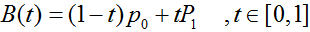
以下公式中:B(t)为t时间下 点的坐标;
P0为起点,Pn为终点,Pi为控制点
一阶贝塞尔曲线(线段):
意义:由 P0 至 P1 的连续点, 描述的一条线段
二阶贝塞尔曲线(抛物线):
原理:由 P0 至 P1 的连续点 Q0,描述一条线段。
由 P1 至 P2 的连续点 Q1,描述一条线段。
由 Q0 至 Q1 的连续点 B(t),描述一条二次贝塞尔曲线。
经验:P1-P0为曲线在P0处的切线。
三阶贝塞尔曲线:
通用公式:
高阶贝塞尔曲线:
4阶曲线:
5阶曲线:
http://www.cs.mtu.edu/~shene/COURSES/cs3621/NOTES/spline/Bezier/de-casteljau.html
Following the construction of a Bézier curve, the next important task is to find the point C(u) on the curve for a particular u. A simple way is to plug u into every basis function, compute the product of each basis function and its corresponding control point, and finally add them together. While this works fine, it is not numerically stable (i.e., could introduce numerical errors during the course of evaluating the Bernstein polynomials).
In what follows, we shall only write down the control point numbers. That is, the control points are 00 for P0, 01 for P1, ..., 0i for Pi, ..., 0n for Pn. The 0s in these numbers indicate the initial or the 0-th iteration. Later on, it will be replaced with 1, 2, 3 and so on.
The fundamental concept of de Casteljau's algorithm is to choose a point C in line segment AB such that C divides the line segment AB in a ratio of u:1-u (i.e., the ratio of the distance between A and C and the distance between A and B is u). Let us find a way to determine the point C.
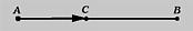
The vector from A to B is B - A. Since u is a ratio in the range of 0 and 1, point C is located at u(B - A). Taking the position of A into consideration, point C is A + u(B - A) = (1 - u)A + uB. Therefore, given a u, (1 - u)A + uB is the point C between A and B that divides AB in a ratio of u:1-u.
The idea of de Casteljau's algorithm goes as follows. Suppose we want to find C(u), where u is in [0,1]. Starting with the first polyline, 00-01-02-03...-0n, use the above formula to find a point 1i on the leg (i.e. line segment) from 0i to0(i+1) that divides the line segment 0i and 0(i+1) in a ratio of u:1-u. In this way, we will obtain n points 10, 11, 12, ...., 1(n-1). They define a new polyline of n - 1 legs.
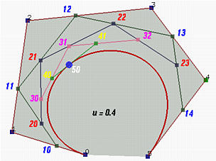
In the figure above, u is 0.4. 10 is in the leg of 00 and 01, 11 is in the leg of 01 and 02, ..., and 14 is in the leg of04 and 05. All of these new points are in blue.
The new points are numbered as 1i's. Apply the procedure to this new polyline and we shall get a second polyline of n - 1 points 20, 21, ..., 2(n-2) and n - 2 legs. Starting with this polyline, we can construct a third one of n - 2 points 30,31, ..., 3(n-3) and n - 3 legs. Repeating this process n times yields a single point n0. De Casteljau proved that this is the point C(u) on the curve that corresponds to u.
Let us continue with the above figure. Let 20 be the point in the leg of 10 and 11 that divides the line segment 10 and 11in a ratio of u:1-u. Similarly, choose 21 on the leg of 11 and 12, 22 on the leg of 12 and 13, and 23 on the leg of 13and 14. This gives a third polyline defined by 20, 21, 22 and 23. This third polyline has 4 points and 3 legs. Keep doing this and we shall obtain a new polyline of three points 30, 31 and 32. From this fourth polyline, we have the fifth one of two points 40 and 41. Do it once more, and we have 50, the point C(0.4) on the curve.
This is the geometric interpretation of de Casteljau's algorithm, one of the most elegant result in curve design.

Actual Computation
Given the above geometric interpretation of de Casteljau's algorithm, we shall present a computation method, which is shown in the following figure.
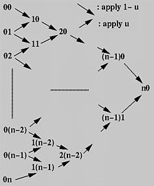
First, all given control points are arranged into a column, which is the left-most one in the figure. For each pair of adjacent control points, draw a south-east bound arrow and a north-east bound arrow, and write down a new point at the intersection of the two adjacent arrows. For example, if the two adjacent points are ij and i(j+1), the new point is(i+1)j. The south-east (resp., north-east) bound arrow means multiplying 1 - u (resp., u) to the point at its tail, ij(resp., i(j+1)), and the new point is the sum.
Thus, from the initial column, column 0, we compute column 1; from column 1 we obtain column 2 and so on. Eventually, aftern applications we shall arrive at a single point n0 and this is the point on the curve. The following algorithm summarizes what we have discussed. It takes an array P of n+1 points and a u in the range of 0 and 1, and returns a point on the Bézier curve C(u).
- Q
i
[
P
] :=
i
[
]; // save input
Input: array P[0:n] of n+1 points and real number u in [0,1]
- Q
i
[
u
] := (1 -
Q
)
i
[
u
] +
Q
i
[
+ 1];
for i := 0 to n - k do
Output: point on curve, C(u)
Working: point array Q[0:n]
for i := 0 to n do
for k := 1 to n do
return Q[0];
A Recurrence Relation
The above computation can be expressed recursively. Initially, let P0,j be Pj for j = 0, 1, ..., n. That is, P0,j is the j-th entry on column 0. The computation of entry j on column i is the following:
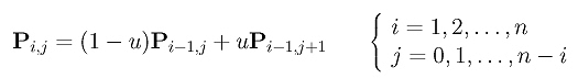
More precisely, entry Pi,j is the sum of (1-u)Pi-1,j (upper-left corner) and uPi-1,j+1 (lower-left corner). The final result (i.e., the point on the curve) is Pn,0. Based on this idea, one may immediately come up with the following recursive procedure:
function deCasteljau(i,j)
- return P0,j
returnu
(1-
deCasteljau
)*
i
(
j
-1,
u
) +
deCasteljau
*
i
(
j
-1,
+1)
if i = 0 then
else
begin
endThis procedure looks simple and short; however, it is extremely inefficient. Here is why. We start with a call todeCasteljau(n,0) for computing Pn,0. The else part splits this call into two more calls, deCasteljau(n-1,0) for computing Pn-1,0 and deCasteljau(n-1,1) for computing Pn-1,1.
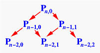
Consider the call to deCasteljau(n-1,0). It splits into two more calls, deCasteljau(n-2,0) for computing Pn-2,0 anddeCasteljau(n-2,1) for computing Pn-2,1. The call to deCasteljau(n-1,1) splits into two calls, deCasteljau(n-2,1) for computing Pn-2,1 and deCasteljau(n-2,2) for computing Pn-2,2. Thus, deCasteljau(n-2,1) is called twice. If we keep expanding these function calls, we should discover that almost all function calls for computing Pi,j are repeated, not once but many times. How bad is this? In fact, the above computation scheme is identical to the following way of computing then-th Fibonacci number:
This program takes an exponential number of function calls (an exercise) to compute Fibonacci(n). Therefore, the above recursive version of de Casteljau's algorithm is not suitable for direct implementation, although it looks simple and elegant!
function Fibonacci(n)
- return
1
returnFibonacci
n
(
Fibonacci
-1) +
n
(
-2)
if n = 0 or n = 1 then
else
beginend
An Interesting Observation
The triangular computation scheme of de Casteljau's algorithm offers an interesting observation. Take a look at the following computation on a Bézier curve of degree 7 defined by 8 control points 00, 01, ..., 07. Let us consider a set of consecutive points on the same column as the control points of a Bézier curve. Then, given a u in [0,1], how do we compute the corresponding point on this Bézier curve? If de Casteljau's algorithm is applied to these control points, the point on the curve is the opposite vertex of the equilateral's base formed by the selected points!
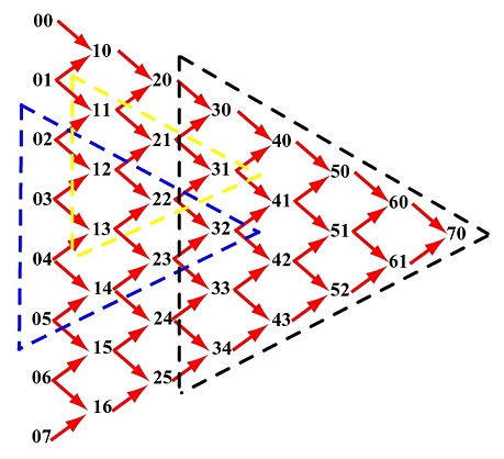
For example, if the selected points are 02, 03, 04 and 05, the point on the curve defined by these four control points that corresponds to u is 32. See the blue triangle. If the selected points are 11, 12 and 13, the point on the curve is31. See the yellow triangle. If the selected points are 30, 31, 32, 33 and 34, the point on the curve is 70.
By the same reason, 70 is the point on the Bézier curve defined by control points 60 and 61. It is also the point on the curve defined by 50, 51 and 52, and on the curve defined by 40, 41, 42 and 43. In general, if we select a point and draw an equilateral as shown above, the base of this equilateral consists of the control points from which the selected point is computed.