
HZNU数模小测试解析
一、填空题
- 在种群增长预测问题中,若资源环境等因素是有限的,则应使用的微分方程模型为 Logistic模型
- 某种群分为 4 个年龄组, 各组的繁殖率分别为 0, 0.8, 1.8, 0.2, 存活率分别为 0.5, 0.7, 0.9, 0. 现各组的数量均为 100, 则该种群的的稳定分布向量为
解:稳定分布向量为矩阵最大特征根所对应的特征向量归一化以后的向量【数学模型P203-206】,下面用R求解
> # --第二题--
> # 构造矩阵L
> L <- matrix(0, ncol = 4, nrow = 4)
> L[1, ] <- c(0, 0.8, 1.8, 0.2)
> L[2, 1] = 0.5
> L[3, 2] = 0.7
> L[4, 3] = 0.9
> eigen(L) -> L.eig
> Re(L.eig$vec[, 1]/sum(L.eig$vec[, 1])) -> w
> w
[1] 0.4769818 0.2307251 0.1562485 0.1360446
于是稳定分布向量为 \((0.4769818, 0.2307251, 0.1562485, 0.1360446)\).
- 工艺品店前段时间的销售额为
19 10 9 11 9 15 12 17 12 10 11 9 12 8 10 11 15 11 10 14 11 15 10 6 16 15 11 16 13 12 11
已知每个工艺品的成本是 300 元,售价是 800 元,但在关店时仍未售出则只能丢弃.若希望收益最大,那么每日制作工艺品数量应为_______.
解:【数学模型P282】
将工艺品的需求视为连续型随机变量,用概率密度函数描述概率分布
> shapiro.test(xse)

	Shapiro-Wilk normality test

data:  xse
W = 0.95367, p-value = 0.197
shapiro检验结果可以认为需求量服从正态分布. 设其平均值为 \(\mu\), 标准差为 \(\sigma\),则需求量为 \(N(\mu,\sigma^2)\)
设每日制作的工业品数量为 \(q\),\(s_1\) 为每日售出一单位工艺品的获利,\(s_2\) 为因未售出而丢弃的一单位工艺品的损失,\(r\) 为某天的需求量. 记需求量的概率密度函数为 \(p(r)\). 于是日均利润为
则要求 \(E(q)\) 最大,令 \(\frac{\mathrm{d}E}{\mathrm{d}q}=0\),记 \(r\) 的概率分布函数为 \(F(q) = \int_{-\infty}^qp(r)\mathrm{d}r\),可得 \(q\) 的最优解满足
根据题意 \(s_1 = 800-300=500,\ s_2 = 300\). 下面用R求q的值
> s1 <- 500
> s2 <- 300
> mean(xse) -> mu
> sd(xse) -> sigma
> f <- s1/(s1+s2)
> qnorm(f, mu, sigma)
[1] 12.89302
故每日制作的最佳工艺品数量为13
二、建模与计算题
- 某阵地(原点)向位于(L,0)处的敌舰发射导弹,敌舰随即以速度(0,v)逃窜。若在任何时刻(位置),导弹的飞行方向都对准敌舰,且速度大于 v,请列出其飞行曲线 y(x)所满足的方
程.
解:记 \(x = x(t),\ y = y(t)\),设导弹合速度为 \(u\),将 \(u\) 分解为水平方向的 \(u_x\) 和竖直方向的 \(u_y\). 示意图如下(有点丑别介意)
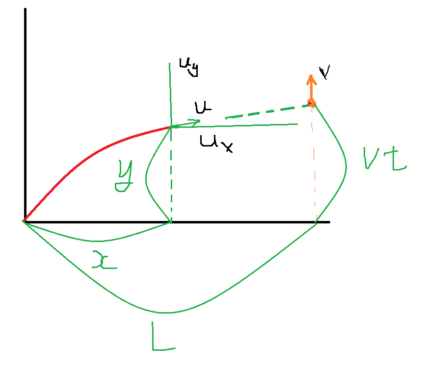
容易列出
- 每隔 1 小时测得的某细菌的生物量数据为:9.6, 18.3, 29.0, 47.2, 71.1, 119.1, 174.6, 257.3, 350.7, 441.0, 513.3, 559.7, 594.8, 629.4, 640.8, 651.1, 655.9, 659.6, 661.8. 试建立 Logistic 模型,并给出下 1 个小时该细菌生物量的预测值
解. 设生物量为 \(x\),生物量增长率为 \(r(x)\),不妨设 \(r(x) = a + bx\). 记 \(x_m\) 为所能容纳的生物量最大值,且当 \(x = x_m\) 时细菌量不再增长;\(r\) 为 \(x=0\) 时的增长率.
于是可以得到 \(a = r, \ b = -\frac{r}{x_m}\). 可以得到 Logistic 模型
那么只需估计出参数 \(x_m\) 和 \(r\) 即可.
- 方法一 线性最小二乘法估计
方程式改写为
R代码:
> # --第二题--
> x <- c(9.6, 18.3, 29.0, 47.2, 71.1, 119.1,
+        174.6, 257.3, 350.7, 441.0, 513.3, 559.7,
+        594.8, 629.4, 640.8, 651.1, 655.9, 659.6, 661.8)
> # 线性最小二乘估计
> # 使用数值微分近似估计增长率
> dx <- c()
> dx[1] <- (-3*x[1]+4*x[2]-x[3])/2
> for (i in 2:(length(x)-1)){
+   dx[i] <- (x[i+1]-x[i-1])/2
+ }
> dx[length(x)] <- (x[length(x)-2]-4*x[length(x)-1]+3*x[length(x)])/2
> xx <- dx/x
> # 最小二乘估计
> lm(xx~x) -> sol2
> summary(sol2)

Call:
lm(formula = xx ~ x)

Residuals:
      Min        1Q    Median        3Q       Max
-0.088687 -0.019463 -0.006286  0.006698  0.234409

Coefficients:
              Estimate Std. Error t value Pr(>|t|)
(Intercept)  5.761e-01  2.579e-02   22.34 4.88e-14 ***
x           -8.780e-04  5.692e-05  -15.43 1.98e-11 ***
---
Signif. codes:  0 ‘***’ 0.001 ‘**’ 0.01 ‘*’ 0.05 ‘.’ 0.1 ‘ ’ 1

Residual standard error: 0.06389 on 17 degrees of freedom
Multiple R-squared:  0.9333,	Adjusted R-squared:  0.9294
F-statistic:   238 on 1 and 17 DF,  p-value: 1.983e-11
> 5.761e-01/8.780e-04
[1] 656.1503
于是 \(r = 0.5761, \ x_m = 656.1503\). 下面用 R 预测
> xm <- 5.761e-01/8.780e-04
> x0 <- 9.6
> r <- 5.761e-01
> f = function(t) xm/(1+(xm/x0-1)*exp(-r*t))
> f((length(x)+1))
[1] 655.7127
故下一个小时的预测值为655.7127.
- 方法二 非线性最小二乘估计
> library(pracma)
> Ffun<-function(y){
+   f<-numeric(length(x))
+   for(i in 1:(length(x))) {
+     f[i]<-x[i]-y[2]/(1+(y[2]/y[1]-1)*exp(-y[3]*(i-1)))
+   }
+   f
+  }
> sol22<-lsqnonlin(Ffun,x0=c(10,666,0.57))
> sol22
$x
[1]   9.1355173 663.0219910   0.5469947

$ssq
[1] 194.3254

$ng
[1] 0.0007158751

$nh
[1] 3.155265e-07

$mu
[1] 0.004704803

$neval
[1] 15

$errno
[1] 1

$errmess
[1] "Stopped by small x-step."
于是 \(r = 0.5469947,\ x_m = 663.0219910\).
预测:
> x0 <- sol22$x[1]
> xm <- sol22$x[2]
> r <- sol22$x[3]
> f(length(x)+1)
[1] 662.1814
故下一个小时的预测值为662.1814.
- 某旅行团计划进行一次假期旅行, 有 4 个备选方案. 已知选择目的地时的参考指标有费
用(万元),景色(分),食宿条件(分),劳累程度(分)四项, 4 处目的地的得分如下表所示. 请使用理想数法选择最适合的目的地.(矩阵标准化时指定使用模一化方法)
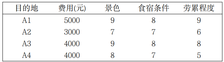
解:先构造决策矩阵,并模一化
由于“费用”和“劳累程度”为费用型属性,因此要取倒数化为效益型属性
R代码:
> # --第三题--
> D <- matrix(c(1/5000, 1/3000, 1/4000, 1/4000,
+               9, 7, 9, 8, 8, 7, 8, 7,
+               1/9, 1/6, 1/8, 1/5), nrow = 4)
> DD <- D^2
> m <- apply(DD, 2, sum)
> m <- sqrt(m)
> M <- matrix(c(m, m, m, m), nrow = 4, byrow = T)
> R <- D/M
> R
          [,1]      [,2]      [,3]      [,4]
[1,] 0.3806169 0.5427204 0.5321521 0.3590803
[2,] 0.6343615 0.4221159 0.4656331 0.5386205
[3,] 0.4757711 0.5427204 0.5321521 0.4039654
[4,] 0.4757711 0.4824182 0.4656331 0.6463446
下面用信息熵计算权重
> xxs <- function(x) -sum(x*log(x))/log(4)
> E <- apply(R, 2, xxs)
> F <- 1 - E
> w <- F/sum(F)
> w
[1] 0.32807915 0.10223509 0.04381521 0.52587055
于是权重为 0.32807915 0.10223509 0.04381521 0.52587055.
下面用Topsis法评价
> # 理想数法
> W <- diag(w)
> V <- R %*% W
> v_max <- apply(V, 2, max)
> v_min <- apply(V, 2, min)
> V_MAX <- matrix(c(v_max, v_max, v_max, v_max), nr = 4, byrow = TRUE)
> V_MIN <- matrix(c(v_min, v_min, v_min, v_min), nr = 4, byrow = TRUE)
> fun <- function(x) sqrt(sum(x^2))
> s_max <- apply(V-V_MAX, 1, fun)
> s_min <- apply(V-V_MIN, 1, fun)
> C <- s_min/(s_max + s_min)
> C
[1] 0.06842871 0.68438747 0.23006165 0.74631797
于是各目的地得分为0.06842871 0.68438747 0.23006165 0.74631797,因此选A4最佳.
- 文件《民航里程数》给出了我国的民航里程数据(见附录 1,民航里程数据),已知民航里程数Y与时间t之间的关系可以近似使用关系式 \(y = k - \frac{k^2}{(\frac{a}{x})^b-2}\)刻画 , 其中k(5<k<100),a(0<a<1),b(0<b<1)为待估参数.请根据样本使用最小二乘法估计这三个参数.
解:利用R求解
> # -- 第四题--
> library(pracma)
> x <- scan("clipboard")
Read 20 items
> f4 <- function(u){
+   f <- numeric(20)
+   for (i in 1:20){
+     f[i] <- x[i] - (u[1]-u[1]^2/((u[2]/i)^u[3]-2))
+   }
+   f
+ }
> sol4 <- lsqnonlin(f4, x0 = c(10, 1, 1))
> sol4
$x
[1] 20.0  0.8  0.6

$ssq
[1] 7.087413e-13

$ng
[1] 1.371535e-05

$nh
[1] 4.710978e-08

$mu
[1] 0.7030284

$neval
[1] 23

$errno
[1] 1

$errmess
[1] "Stopped by small x-step."
于是 \(a = 0.8,\ b = 0.6, \ k=20\).
- 某地区进行了用电量调查,得到的数据(见附录 2,高峰用电量与总用电量数据),其中X代表每月用电量,Y 代表高峰时期每小时的用电量。
(1)利用样本数据, 以 Y 为因变量,X 为自变量建立线性回归方程拟合两者的关系,并对所得
回归方程进行显著性检验。
(2)若根据历史资料估计, 7 月份的平均用电量为 2000,试估计该月份的用电高峰时期每小时用电量,并求其 95%置信区间.
解:
(1)利用R求解
> # -- 第五题 --
> t5 <- read.table("clipboard", header = T)
> t5
      X    Y
1   679   79
2   292   44
3  1012   56
4   493   79
5   582  270
6  1156  364
7   997  473
8  2189  950
9  1097  534
10 2078  685
11 1818  584
12 1700  521
13  747  325
14 2030  443
15 1643  316
16  414   50
17  354   17
18 1276  188
19  745   77
20  435  139
21  540   56
22  874  156
23 1543  528
24 1029   64
25  710  400
26 1434   31
27  837  420
28 1748  488
29 1381  348
30 1428  758
31 1255  263
32 1777  499
33  370   59
34 2316  819
35 1130  479
36  463   51
37  770  174
38  724  410
39  808  394
40  790   96
41  783  329
42  406   44
43 1242  324
44  658  214
45 1746  571
46  468   64
47 1114  190
48  413   51
49 1787  833
50 3560 1494
51 1495  511
52 2221  385
53 1526  393
> x <- t5$X
> y <- t5$Y
> lm(y~x) -> sol5
> summary(sol5)

Call:
lm(formula = y ~ x)

Residuals:
    Min      1Q  Median      3Q     Max
-413.99  -82.75  -19.34  123.76  315.22

Coefficients:
             Estimate Std. Error t value Pr(>|t|)
(Intercept) -83.13037   44.16121  -1.882   0.0655 .
x             0.36828    0.03339  11.030 4.11e-15 ***
---
Signif. codes:
0 ‘***’ 0.001 ‘**’ 0.01 ‘*’ 0.05 ‘.’ 0.1 ‘ ’ 1

Residual standard error: 157.7 on 51 degrees of freedom
Multiple R-squared:  0.7046,	Adjusted R-squared:  0.6988
F-statistic: 121.7 on 1 and 51 DF,  p-value: 4.106e-15
#常数项未通过检验,置为0
> lm(y~0+x) -> sol51
> summary(sol51)

Call:
lm(formula = y ~ 0 + x)

Residuals:
    Min      1Q  Median      3Q     Max
-418.58 -113.30  -58.11   87.54  377.89

Coefficients:
  Estimate Std. Error t value Pr(>|t|)
x  0.31351    0.01678   18.69   <2e-16 ***
---
Signif. codes:  0 ‘***’ 0.001 ‘**’ 0.01 ‘*’ 0.05 ‘.’ 0.1 ‘ ’ 1

Residual standard error: 161.5 on 52 degrees of freedom
Multiple R-squared:  0.8704,	Adjusted R-squared:  0.8679
F-statistic: 349.2 on 1 and 52 DF,  p-value: < 2.2e-16
于是
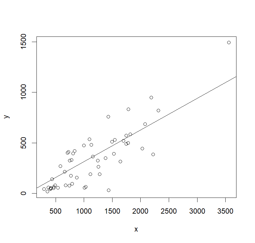
且检验统计量 \(F = 349.2, \ p << 0.01\),因此认为两者具有显著的线性关系,\(R^2 = 0.8704\) 说明拟合程度较好.
来看看拟合效果
> plot(x,y)
> abline(sol51)
(2) R 程序如下
> x0 <- data.frame(x = 2000)
> Pred <- predict(sol51, x0, interval = "confidence", level = 0.95)
> Pred
       fit   lwr      upr
1 627.0274 559.7 694.3549
于是得到高峰用电量为627.0274,其置信区间为 (559.7, 694.3549).
- 求解下面二次规划问题:
请写出(lingo 或者 R 或者 matlab)程序和计算结果。
解:规划问题用Lingo求解比较方便,考虑使用Lingo求解
model:

min = x1^2 + x2^2 - 2*x1 - 5*x2;

x1 - 2*x2 >= -2;

-x1 - 2*x2 >= -6;

-x1 + 2*x2 >= -2;

end
输出:
Global optimal solution found.
  Objective value:                             -6.450000
  Objective bound:                             -6.450000
  Infeasibilities:                              0.000000
  Extended solver steps:                               0
  Total solver iterations:                             8
  Elapsed runtime seconds:                          0.11
  Model is convex quadratic

  Model Class:                                        QP

  Total variables:                      2
  Nonlinear variables:                  2
  Integer variables:                    0

  Total constraints:                    4
  Nonlinear constraints:                1

  Total nonzeros:                       8
  Nonlinear nonzeros:                   2


                                Variable           Value        Reduced Cost
                                      X1        1.400002            0.000000
                                      X2        1.700001            0.000000

                                     Row    Slack or Surplus      Dual Price
                                       1       -6.450000           -1.000000
                                       2        0.000000          -0.8000000
                                       3        1.199997            0.000000
                                       4        4.000000            0.000000
于是目标最小值为-6.45,其中 \(x_1 = 1.4,x_2=1.7\).
- 考虑 3 个产地与 4 个销地的问题,各产地的产量、各销地的销量及各产地到各销地的单 位运费如下表。问如何调运,才可使总的运费最少?请根据问题建立数学模型。
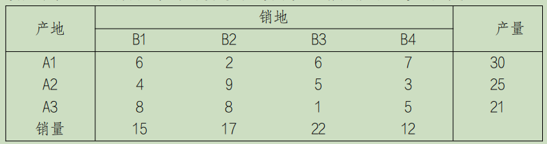
解:7. 发现产销不平衡,产量(76)>销量(66),因此假想一个销地 B5,各产地到B5的运费为0且销量为10.
设Ai到Bj的运量为 \(x_{ij}\),运费矩阵为
使用Lingo求解
代码:
model:

sets:

thr /1..3/ : cl;
fiv /1..5/ : xl;
coor(thr,fiv) : A, x;

endsets

data:

cl = 30, 25, 21;
xl = 15, 17, 22, 12, 10;
A = 6, 2, 6, 7, 0
    4, 9, 5, 3, 0
    8, 8, 1, 5, 0;

enddata

min = @sum(coor(i, j): A(i,j)*x(i,j));

@for(thr(i) : @sum(fiv(j) : x(i,j)) = cl(i));

@for(fiv(j) : @sum(thr(i) : x(i,j)) = xl(j));

end
输出:
  Global optimal solution found.
  Objective value:                              161.0000
  Infeasibilities:                              0.000000
  Total solver iterations:                             8
  Elapsed runtime seconds:                          0.05

  Model Class:                                        LP

  Total variables:                     15
  Nonlinear variables:                  0
  Integer variables:                    0

  Total constraints:                    9
  Nonlinear constraints:                0

  Total nonzeros:                      42
  Nonlinear nonzeros:                   0

                                Variable           Value        Reduced Cost
                                  CL( 1)        30.00000            0.000000
                                  CL( 2)        25.00000            0.000000
                                  CL( 3)        21.00000            0.000000
                                  XL( 1)        15.00000            0.000000
                                  XL( 2)        17.00000            0.000000
                                  XL( 3)        22.00000            0.000000
                                  XL( 4)        12.00000            0.000000
                                  XL( 5)        10.00000            0.000000
                                A( 1, 1)        6.000000            0.000000
                                A( 1, 2)        2.000000            0.000000
                                A( 1, 3)        6.000000            0.000000
                                A( 1, 4)        7.000000            0.000000
                                A( 1, 5)        0.000000            0.000000
                                A( 2, 1)        4.000000            0.000000
                                A( 2, 2)        9.000000            0.000000
                                A( 2, 3)        5.000000            0.000000
                                A( 2, 4)        3.000000            0.000000
                                A( 2, 5)        0.000000            0.000000
                                A( 3, 1)        8.000000            0.000000
                                A( 3, 2)        8.000000            0.000000
                                A( 3, 3)        1.000000            0.000000
                                A( 3, 4)        5.000000            0.000000
                                A( 3, 5)        0.000000            0.000000
                                X( 1, 1)        2.000000            0.000000
                                X( 1, 2)        17.00000            0.000000
                                X( 1, 3)        1.000000            0.000000
                                X( 1, 4)        0.000000            2.000000
                                X( 1, 5)        10.00000            0.000000
                                X( 2, 1)        13.00000            0.000000
                                X( 2, 2)        0.000000            9.000000
                                X( 2, 3)        0.000000            1.000000
                                X( 2, 4)        12.00000            0.000000
                                X( 2, 5)        0.000000            2.000000
                                X( 3, 1)        0.000000            7.000000
                                X( 3, 2)        0.000000            11.00000
                                X( 3, 3)        21.00000            0.000000
                                X( 3, 4)        0.000000            5.000000
                                X( 3, 5)        0.000000            5.000000

                                     Row    Slack or Surplus      Dual Price
                                       1        161.0000           -1.000000
                                       2        0.000000           -2.000000
                                       3        0.000000            0.000000
                                       4        0.000000            3.000000
                                       5        0.000000           -4.000000
                                       6        0.000000            0.000000
                                       7        0.000000           -4.000000
                                       8        0.000000           -3.000000
                                       9        0.000000            2.000000
于是方案为:
| 产地/销地 | B1 | B2 | B3 | B4 | 产量 |
|---|---|---|---|---|---|
| A1 | 2 | 17 | 1 | 0 | 30 |
| A2 | 13 | 0 | 0 | 12 | 25 |
| A3 | 0 | 0 | 21 | 0 | 21 |
| 销量 | 15 | 17 | 22 | 12 |
费用最小为161.
- 某工厂生产 A,B,C 三种产品,其所需劳动力、材料等有关数据如下表所示.(1)确定获利最 大的生产方案;(2)产品 A,B,C 的利润分别在什么范围内变动时,上述最优方案不变;(3)如果劳动 力数量不增,材料不足可以从市场购买,每单位0.4元,问该厂要不要购进原材料扩大生产,购买 多少为宜?(要求给出数学模型以及相关的程序 lingo 或者 R 或者 matlab)
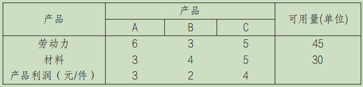
解:(1)设生产A,B,C产量分别为 \(x_1,x_2,x_3\) , \(z\) 为目标,可得如下模型:
使用Lingo求解
代码:
model:

max = 3*x1+2*x2+4*x3;

6*x1+3*x2+5*x3<=45;

3*x1+4*x2+5*x3<=30;

end
输出结果为:
Global optimal solution found.
      Objective value:                              27.00000
      Infeasibilities:                              0.000000
      Total solver iterations:                             2
      Elapsed runtime seconds:                          0.05

      Model Class:                                        LP

      Total variables:                      3
      Nonlinear variables:                  0
      Integer variables:                    0

      Total constraints:                    6
      Nonlinear constraints:                0

      Total nonzeros:                      12
      Nonlinear nonzeros:                   0


                                    Variable           Value        Reduced Cost
                                          X1        5.000000            0.000000
                                          X2        0.000000            1.000000
                                          X3        3.000000            0.000000

                                         Row    Slack or Surplus      Dual Price
                                           1        27.00000            1.000000
                                           2        0.000000           0.2000000
                                           3        0.000000           0.6000000
                                           4        5.000000            0.000000
                                           5        0.000000            0.000000
                                           6        3.000000            0.000000
故最优方案为:生产5个A,0个B,3个C,且获利最大为27.
(2) 灵敏度分析可得
Ranges in which the basis is unchanged:

                                       Objective Coefficient Ranges:

                                        Current        Allowable        Allowable
                      Variable      Coefficient         Increase         Decrease
                            X1         3.000000         1.800000        0.6000000
                            X2         2.000000         1.000000         INFINITY
                            X3         4.000000         1.000000         1.000000

                                           Righthand Side Ranges:

                                        Current        Allowable        Allowable
                           Row              RHS         Increase         Decrease
                             2         45.00000         15.00000         15.00000
                             3         30.00000         15.00000         7.500000
则A的范围为 \([2.4,4.8]\),B的范围为 \((-\infty,3.0]\),C的范围为 \([3.0,5.0]\),最优方案不变.
(3) 设购买原材料数量为\(x_4\).
模型改为
使用Lingo求解
代码:
model:

max = 3*x1+2*x2+4*x3-0.4*x4;
6*x1+3*x2+5*x3 <= 45;
30+x4 = 3*x1+4*x2+5*x3;

end
输出结果为:
      Global optimal solution found.
      Objective value:                              30.00000
      Infeasibilities:                              0.000000
      Total solver iterations:                             1
      Elapsed runtime seconds:                          0.04

      Model Class:                                        LP

      Total variables:                      4
      Nonlinear variables:                  0
      Integer variables:                    0

      Total constraints:                    7
      Nonlinear constraints:                0

      Total nonzeros:                      15
      Nonlinear nonzeros:                   0


                                    Variable           Value        Reduced Cost
                                          X1        0.000000           0.6000000
                                          X2        0.000000           0.8000000
                                          X3        9.000000            0.000000
                                          X4        15.00000            0.000000

                                         Row    Slack or Surplus      Dual Price
                                           1        30.00000            1.000000
                                           2        0.000000           0.4000000
                                           3        0.000000          -0.4000000
                                           4        0.000000            0.000000
                                           5        0.000000            0.000000
                                           6        9.000000            0.000000
                                           7        15.00000            0.000000
故购买原材料15个最合适,利润最大为30.

