Deep Learning 12_深度学习UFLDL教程：Sparse Coding_exercise（斯坦福大学深度学习教程）

前言

理论知识：UFLDL教程、Deep learning：二十六(Sparse coding简单理解)、Deep learning：二十七(Sparse coding中关于矩阵的范数求导)、Deep learning：二十九(Sparse coding练习)

实验环境：win7， matlab2015b，16G内存，2T机械硬盘

本节实验比较不好理解也不好做，我看很多人最后也没得出好的结果，所以得花时间仔细理解才行。

实验内容：Exercise:Sparse Coding。从10张512*512的已经白化后的灰度图像（即：Deep Learning 一_深度学习UFLDL教程：Sparse Autoencoder练习（斯坦福大学深度学习教程）中用到的数据 sparseae_exercise.zip中的IMAGES.mat）中随机抽取20000张小图像块（大小为8*8或16*16），分别通过稀疏编码（Sparse Coding）和拓扑稀疏编码（topographic sparse coding）的方法学习它们的特征，并分别显示出来。

实验基础说明：

1.稀疏自动编码器（Sparse Autoencoder）和稀疏编码（Sparse Coding）的区别？

①Ng的解释：稀疏编码可以看作是稀疏自编码方法的一个变形，稀疏编码在试图直接学习数据的特征集。而稀疏自动编码是直接学习原始数据。

稀疏编码算法是一种无监督学习方法，它用来寻找一组“超完备”基向量来更高效地表示样本数据，这个“超完备”基的维数大于原始数据的维数。而只有一层隐含层的稀疏自动编码器相当于PCA，只能使我们方便地找到一组“完备”基向量，它的维数小于原始数据的维数。

②稀疏编码算法的目的就是找到一组基向量 $\mathbf{\phi}_i$ ，使得我们能将输入向量 $\mathbf{x}$ 表示为这些基向量的线性组合：

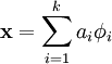　　　　　　　　　　　　　　　　　　　　　　 $\begin{align} \mathbf{x} = \sum_{i=1}^k a_i \mathbf{\phi}_{i} \end{align}$ ，其中x＝[x1,x2,x3，……，xn]

一般情况下要求基的个数k非常大，至少要比x中元素的个数n要大，因此上面这样的方程就大多情况会有无穷多个解。我们为什么要寻找这样的“超完备”基呢？因为超完备基的好处是它们能更有效地找出隐含在输入数据内部的结构与模式。其实在常见的PCA算法中，是可以找到一组基来分解X的，只不过那个基的数目比较小，所以可以得到分解后的系数a是可以唯一确定，而在sparse coding中，k太大，比n大很多，其分解系数a不能唯一确定。为了能唯一确定a，一般的做法是对系数a作一个稀疏性约束，即：要求系数 $a i 是稀疏的。也就是说要求：对于一组输入向量，在a中我们只想有尽可能少的几个系数远大于零，其他都等于0或接近于0。a变稀疏从而就会使x变得稀疏。$

$\mathbf{\phi}_i$

$③ 在稀疏编码中，权值矩阵 A 用于将特征 s 映射到原始数据x，而在以前的所有实验（包括稀疏自动编码）中，权值矩阵 W 工作的方向相反，是将原始数据 x 映射到特征$

2.稀疏编码的作用？即：为什么要稀疏编码？

Ng已经回答了：稀疏编码算法是一种无监督学习方法，它用来寻找一组“超完备”基向量来更高效地表示样本数据，而超完备基的好处是它们能更有效地找出隐含在输入数据内部的结构与模式。

3.代价函数

非拓扑稀疏编码（non-topographic sparse coding）时的代价函数：

拓扑稀疏编码（topographic sparse coding）时的代价函数：

注意： $\lVert x \rVert_k$ 是x的Lk范数，等价于 $\left( \sum{ \left| x_i^k \right| } \right) ^{\frac{1}{k}}$ 。L2 范数即大家熟知的欧几里得范数，即：平方和的开方。L1 范数是向量元素的绝对值之和

在Ng的讲解中，这个代价函数表达是不准确的，起码在重构项中少了要除以元素个数，即：重构项实际上是均方误差，而不是误差平方和。

4.代价函数的导数

代价函数关于权值矩阵A的导数（拓扑和非拓扑时结果是一样的，因为此时这2种情况下代价函数关于A是没区别的）：

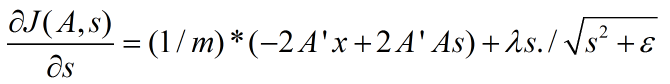
非拓扑稀疏编码（non-topographic sparse coding）时代价函数关于s的导数：

拓扑稀疏编码（topographic sparse coding）时代价函数关于s的导数为：

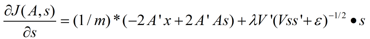
其中，m为样本数量。

上面矩阵求导公式的推导，可参考Deep learning：二十七(Sparse coding中关于矩阵的范数求导)、http://www.mathchina.net/dvbbs/dispbbs.asp?boardid=4&Id=3673和The Matrix Cookbook（强烈推荐这本书，还有Writing Fast MATLAB Code (by Pascal Getreuer)也非常值得一看）。

5.迭代优化时的参数

迭代优化参数时，给定s优化A时，由于A有直接的解析解，所以不需要通过lbfgs等优化算法求得，通过令代价函数对A的导函数为0，可以得到解析解为：

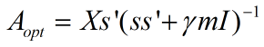　　其中，m为样本个数。

6.注意理解：本节实验的代价函数是怎么推导出来的？只有在理解它的基础上，以后才能自己根据自己的模型和需要来推导自己的代价函数。

实际上，Ng在他的讲解（稀疏编码和稀疏编码自编码表达）中已经很详细清楚地讲明了这一点。下面的解释只是为了把话说得更直白一点：

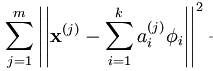
①重构项：因为本节实验的目的是寻找数据X的“超完备”基，并把数据x用“超完备”基表示出来，即： $\begin{align} \mathbf{x} = \sum_{i=1}^k a_i \mathbf{\phi}_{i} \end{align}$ ，其中 $\mathbf{\phi}_i$ 就是它的“超完备”基，其矩阵表示为A。 $a i 是数据x的特征集（也就是“超完备”基的系数），其矩阵表示为s。$

$为了使数据x和之间的误差最小，那么代价函数必须要包括这两者的均方差，并且要使这个代价函数最小，即：$

$最小化，$

$矩阵表示为：$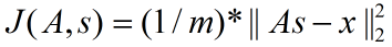

$Ng叫这一项为“重构项”，其实也是均方误差项。所以Ng的表示实际上是有一点不准确的，少了除以样本数m，当然这只是表示的问题，在他的代码中是除以m的。$

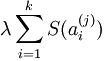$\mathbf{x}$ $，其中在本节实验中 S (.) 的选择是 L 1 范式代价函数，其实也可以选择对数代价函数。$

$只要上式最小化就能保证系数 a i 只有很少的几个远大于零的元素，即保证系数 a i 的稀疏性。因为 a i 的矩阵表示为s，所以稀疏惩罚项矩阵表示为：$

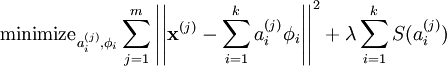
又因为以后我们为求代价函数的最小值，会对代价函数求导，而对s在0点处不可导的（理解：y=|x|在x=0处不可导），所以为了方便以后求代价函数最小值，可把替换为，其中 $ε 是“平滑参数”（"smoothing parameter"）或者“稀疏参数”（"sparsity parameter"）。$

$综上，稀疏惩罚项为：$

故此时代价函数为：

$\begin{align} \text{minimize}_{a^{(j)}_i,\mathbf{\phi}_{i}} \sum_{j=1}^{m} \left|\left| \mathbf{x}^{(j)} - \sum_{i=1}^k a^{(j)}_i \mathbf{\phi}_{i}\right|\right|^{2} + \lambda \sum_{i=1}^{k}S(a^{(j)}_i) \end{align}$ ，

矩阵表示为：

$\mathbf{\phi}_i$

$，矩阵表示为：，$

$\sum_r{\sum_c{A_{rc}^2}}$ $就可以保证前面提到的情况不会发生。$

所以，代价函数第三项为：

$通过这上面三步的推导，我们才得出满足我们要求的代价函数：$

对于拓扑稀疏编码的代价函数可见Ng的解释，他已经说很清楚很好理解了。

7.注意：因为10张512*512的灰度图像是已经白化后的图像，故它的值不是在[0，1]之间。以前实验的sampleIMAGES函数中要把样本归一化到[0，1]之间的原因在于它们都是输入到稀疏自动编码器，其要求输入数据为[0，1]范围，而本节实验是把数据输入到稀疏编码中，它并不要求数据输入范围为[0，1]，同时归一化本身实际上是有误差的（因为它是根据3sigma法则归一化的），所以本节实验修改后的sampleIMAGES函数中，不需要再把随机抽取20000张小图像块归一化到[0，1]范围，即：要把原来sampleIMAGES函数中如下代码注释掉：patches = normalizeData(patches);。实际上这一步非常重要，因为它直接关系到最后是否可以得到要求的结果图。具体抽取函数 sampleIMAGES见下面代码。

8.优秀的编程技巧：

assert(diff < 1e-8, 'Weight difference too large. Check your weight cost function. ');

用于检查逻辑不等式diff < 1e-8为真还是假，如为假就显示：Weight difference too large. Check your weight cost function

9.一些Matlab函数：

　　circshift:

　　该函数是将矩阵循环平移的函数，比如说B = circshift(A,shiftsize)是将矩阵A按照shiftsize的方式左右平移，一般hiftsize为一个多维的向量，第一个元素表示上下方向移动（更准确的说是在第一个维度上移动，这里只是考虑是2维矩阵的情况，后面的类似），如果为正表示向下移，第二个元素表示左右方向移动，如果向右表示向右移动。

　　rndperm：

　　该函数是随机产生一个行向量，比如randperm(n)产生一个n维的行向量，向量元素值为1~n，随机选取且不重复。而randperm(n,k)表示产生一个长为k的行向量，其元素也是在1到n之间，不能有重复。

　　questdlg：

　　button = questdlg('qstring','title','str1','str2','str3',default)，这是一个对话框，对话框中的内容用qstring表示，标题为title，然后后面3个分别为对应yes,no,cancel按钮，最后的参数default为默认的对应按钮。

疑问

1.分组矩阵V究竟应该怎么样产生？为什么这样产生？

Ng对分组矩阵V的产生方法如下：

donutDim = floor(sqrt(numFeatures));
assert(donutDim * donutDim == numFeatures,'donutDim^2 must be equal to numFeatures');

groupMatrix = zeros(numFeatures, donutDim, donutDim);

groupNum = 1;
for row = 1:donutDim
    for col = 1:donutDim
        groupMatrix(groupNum, 1:poolDim, 1:poolDim) = 1;
        groupNum = groupNum + 1;
        groupMatrix = circshift(groupMatrix, [0 0 -1]);
    end
    groupMatrix = circshift(groupMatrix, [0 -1, 0]);
end
%poolDim = 3;

为什么这么产生？没搞懂！

实验步骤

1.初始化参数，然后加载数据（即：10张512*512的已经白化后的灰度图），然后从中随机抽取出20000张小图像块。对于本节修改后的抽取函数见 sampleIMAGES.m。

2. 实现稀疏编码代价函数，并求出代价函数对权值矩阵A的导数，即代价函数对A梯度，然后检查它的实现是否正确。因为非拓扑稀疏编码代价函数和拓扑稀疏编码代价函数对A的导数是一样的，所以这里不用分开求。

3.实现非拓扑稀疏编码代价函数，并求出它对特征集s的导数，即代价函数对s梯度，然后检查它的实现是否正确。

4.实现拓扑稀疏编码代价函数，并求出它对特征集s的导数，即代价函数对s梯度，然后检查它的实现是否正确。

5.迭代优化参数A和s（可用lbfgs或cg算法），得到最佳的权值矩阵A，并把它显示出来。

结果

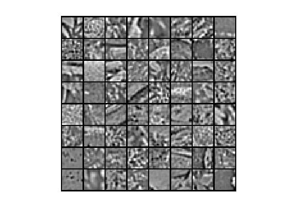
①部分原始数据

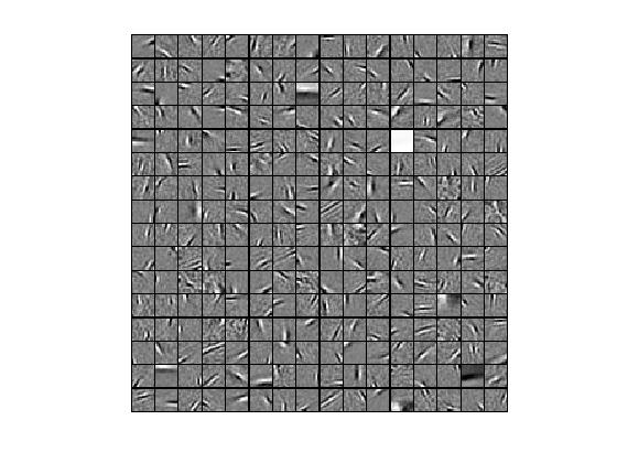
②非拓扑稀疏编码算法，优化算法为lbfgs，特征个数为256，小图像块大小为16*16时，提取的“超完备”基为：

③拓扑稀疏编码算法，优化算法为lbfgs，特征个数为256，小图像块大小为16*16时，提取的“超完备”基为：

④拓扑稀疏编码算法，优化算法为cg，特征个数为256，小图像块大小为16*16时，提取的“超完备”基为：

⑤拓扑稀疏编码算法，优化算法为cg，特征个数为121，小图像块大小为8*8时，提取的“超完备”基为：

总结

1.优化算法对结果是有影响的。比如，从上面可看出，对于拓扑稀疏编码，优化算法为cg，特征个数为121，小图像块大小为16*16时，cg算法得到的结果比lbfgs算法更好。

2.小图像块大小对结果是有影响的。比如，拓扑稀疏编码算法，特征个数为121，小图像块大小为8*8时，如果用lbfgs算法就得不到结果，而用cg算法就可以得到上面的结果。

3.规律：随着迭代次数的增加，代价函数值应该是越来越小的，如果不是，就永远不会得到正确结果。如果代价函数不是越来越小，可能是优化算法的选择有问题，或者小图像块的选择有问题，具体情况具体分析，有多种原因。当然更本质的原因，还没弄清楚。

代码

sparseCodingExercise.m

%% CS294A/CS294W Sparse Coding Exercise

%  Instructions
%  ------------
% 
%  This file contains code that helps you get started on the
%  sparse coding exercise. In this exercise, you will need to modify
%  sparseCodingFeatureCost.m and sparseCodingWeightCost.m. You will also
%  need to modify this file, sparseCodingExercise.m slightly.

% Add the paths to your earlier exercises if necessary
% addpath /path/to/solution
addpath minFunc/;
%%======================================================================
%% STEP 0: Initialization
%  Here we initialize some parameters used for the exercise.

numPatches = 20000;   % number of patches
numFeatures = 256;    % number of features to learn
patchDim = 16;         % patch dimension
visibleSize = patchDim * patchDim; 

% dimension of the grouping region (poolDim x poolDim) for topographic sparse coding
poolDim = 3;

% number of patches per batch
batchNumPatches = 2000; 

lambda = 5e-5;  % L1-regularisation parameter (on features)
epsilon = 1e-5; % L1-regularisation epsilon |x| ~ sqrt(x^2 + epsilon)
gamma = 1e-2;   % L2-regularisation parameter (on basis)

%%======================================================================
%% STEP 1: Sample patches

images = load('IMAGES.mat');
images = images.IMAGES;

patches = sampleIMAGES(images, patchDim, numPatches);
display_network(patches(:, 1:64));

%%======================================================================
%% STEP 2: Implement and check sparse coding cost functions
%  Implement the two sparse coding cost functions and check your gradients.
%  The two cost functions are
%  1) sparseCodingFeatureCost (in sparseCodingFeatureCost.m) for the features 
%     (used when optimizing for s, which is called featureMatrix in this exercise) 
%  2) sparseCodingWeightCost (in sparseCodingWeightCost.m) for the weights
%     (used when optimizing for A, which is called weightMatrix in this exericse)

% We reduce the number of features and number of patches for debugging
debug = false;
if debug
numFeatures = 5;
patches = patches(:, 1:5);
numPatches = 5;

weightMatrix = randn(visibleSize, numFeatures) * 0.005;
featureMatrix = randn(numFeatures, numPatches) * 0.005;

%% STEP 2a: Implement and test weight cost
%  Implement sparseCodingWeightCost in sparseCodingWeightCost.m and check
%  the gradient

[cost, grad] = sparseCodingWeightCost(weightMatrix, featureMatrix, visibleSize, numFeatures, patches, gamma, lambda, epsilon);

numgrad = computeNumericalGradient( @(x) sparseCodingWeightCost(x, featureMatrix, visibleSize, numFeatures, patches, gamma, lambda, epsilon), weightMatrix(:) );
% Uncomment the blow line to display the numerical and analytic gradients side by side
% disp([numgrad grad]);     
diff = norm(numgrad-grad)/norm(numgrad+grad);
fprintf('Weight difference: %g\n', diff);
assert(diff < 1e-8, 'Weight difference too large. Check your weight cost function. ');

%% STEP 2b: Implement and test feature cost (非拓扑结构non-topographic)
%  Implement sparseCodingFeatureCost in sparseCodingFeatureCost.m and check
%  the gradient. You may wish to implement the non-topographic version of
%  the cost function first, and extend it to the topographic version later.

% Set epsilon to a larger value so checking the gradient numerically makes sense
epsilon = 1e-2;

% We pass in the identity matrix as the grouping matrix, putting each
% feature in a group on its own.
groupMatrix = eye(numFeatures);

[cost, grad] = sparseCodingFeatureCost(weightMatrix, featureMatrix, visibleSize, numFeatures, patches, gamma, lambda, epsilon, groupMatrix);

numgrad = computeNumericalGradient( @(x) sparseCodingFeatureCost(weightMatrix, x, visibleSize, numFeatures, patches, gamma, lambda, epsilon, groupMatrix), featureMatrix(:) );
% Uncomment the blow line to display the numerical and analytic gradients side by side
% disp([numgrad grad]); 
diff = norm(numgrad-grad)/norm(numgrad+grad);
fprintf('Feature difference (non-topographic): %g\n', diff);
assert(diff < 1e-8, 'Feature difference too large. Check your feature cost function. ');

%% STEP 2c: Implement and test feature cost (拓扑结构topographic)
%  Implement sparseCodingFeatureCost in sparseCodingFeatureCost.m and check
%  the gradient. This time, we will pass a random grouping matrix in to
%  check if your costs and gradients are correct for the topographic
%  version.

% Set epsilon to a larger value so checking the gradient numerically makes sense
epsilon = 1e-2;

% This time we pass in a random grouping matrix to check if the grouping is
% correct.
groupMatrix = rand(100, numFeatures);

[cost, grad] = sparseCodingFeatureCost(weightMatrix, featureMatrix, visibleSize, numFeatures, patches, gamma, lambda, epsilon, groupMatrix);

numgrad = computeNumericalGradient( @(x) sparseCodingFeatureCost(weightMatrix, x, visibleSize, numFeatures, patches, gamma, lambda, epsilon, groupMatrix), featureMatrix(:) );
% Uncomment the blow line to display the numerical and analytic gradients side by side
% disp([numgrad grad]); 
diff = norm(numgrad-grad)/norm(numgrad+grad);
fprintf('Feature difference (topographic): %g\n', diff);
assert(diff < 1e-8, 'Feature difference too large. Check your feature cost function. ');
end

%%======================================================================
%% STEP 3: Iterative optimization
%  Once you have implemented the cost functions, you can now optimize for
%  the objective iteratively. The code to do the iterative optimization 
%  using mini-batching and good initialization of the features has already
%  been included for you. 
% 
%  However, you will still need to derive and fill in the analytic solution 
%  for optimizing the weight matrix given the features. 
%  Derive the solution and implement it in the code below, verify the
%  gradient as described in the instructions below, and then run the
%  iterative optimization.


% Initialize options for minFunc
options.Method = 'lbfgs';
options.display = 'off';
options.verbose = 0;

% Initialize matrices
weightMatrix = rand(visibleSize, numFeatures);
featureMatrix = rand(numFeatures, batchNumPatches);

% Initialize grouping matrix
assert(floor(sqrt(numFeatures)) ^2 == numFeatures, 'numFeatures should be a perfect square');
donutDim = floor(sqrt(numFeatures));
assert(donutDim * donutDim == numFeatures,'donutDim^2 must be equal to numFeatures');

groupMatrix = zeros(numFeatures, donutDim, donutDim);

groupNum = 1;
for row = 1:donutDim
    for col = 1:donutDim
        groupMatrix(groupNum, 1:poolDim, 1:poolDim) = 1;
        groupNum = groupNum + 1;
        groupMatrix = circshift(groupMatrix, [0 0 -1]);
    end
    groupMatrix = circshift(groupMatrix, [0 -1, 0]);
end

groupMatrix = reshape(groupMatrix, numFeatures, numFeatures);
if isequal(questdlg('Initialize grouping matrix for topographic or non-topographic sparse coding?', 'Topographic/non-topographic?', 'Non-topographic', 'Topographic', 'Non-topographic'), 'Non-topographic')
    groupMatrix = eye(numFeatures);
end

% Initial batch
indices = randperm(numPatches);
indices = indices(1:batchNumPatches);
batchPatches = patches(:, indices);                           

fprintf('%6s%12s%12s%12s%12s\n','Iter', 'fObj','fResidue','fSparsity','fWeight');

for iteration = 1:200                      
    error = weightMatrix * featureMatrix - batchPatches;
    error = sum(error(:) .^ 2) / batchNumPatches;
    
    fResidue = error;
    
    R = groupMatrix * (featureMatrix .^ 2);
    R = sqrt(R + epsilon);    
    fSparsity = lambda * sum(R(:));    
    
    fWeight = gamma * sum(weightMatrix(:) .^ 2);
    
    fprintf('  %4d  %10.4f  %10.4f  %10.4f  %10.4f\n', iteration, fResidue+fSparsity+fWeight, fResidue, fSparsity, fWeight)
               
    % Select a new batch
    indices = randperm(numPatches);
    indices = indices(1:batchNumPatches);
    batchPatches = patches(:, indices);                    
    
    % Reinitialize featureMatrix with respect to the new batch
    featureMatrix = weightMatrix' * batchPatches;
    normWM = sum(weightMatrix .^ 2)';
    featureMatrix = bsxfun(@rdivide, featureMatrix, normWM); 
    
    % Optimize for feature matrix    
    options.maxIter = 20;
    [featureMatrix, cost] = minFunc( @(x) sparseCodingFeatureCost(weightMatrix, x, visibleSize, numFeatures, batchPatches, gamma, lambda, epsilon, groupMatrix), ...
                                           featureMatrix(:), options);
    featureMatrix = reshape(featureMatrix, numFeatures, batchNumPatches);                                      
       
    % Optimize for weight matrix  
%     weightMatrix = zeros(visibleSize, numFeatures);     
    % -------------------- YOUR CODE HERE --------------------
    % Instructions:
    %   Fill in the analytic solution for weightMatrix that minimizes 
    %   the weight cost here.     
    %   Once that is done, use the code provided below to check that your
    %   closed form solution is correct.
    %   Once you have verified that your closed form solution is correct,
    %   you should comment out the checking code before running the
    %   optimization.
    
    weightMatrix = batchPatches * featureMatrix' / (featureMatrix * featureMatrix' + gamma * batchNumPatches * eye(numFeatures));
    
%     [cost, grad] = sparseCodingWeightCost(weightMatrix, featureMatrix, visibleSize, numFeatures, batchPatches, gamma, lambda, epsilon, groupMatrix);
%     assert(norm(grad) < 1e-12, 'Weight gradient should be close to 0. Check your closed form solution for weightMatrix again.')
%     error('Weight gradient is okay. Comment out checking code before running optimization.');
    % -------------------- YOUR CODE HERE --------------------   
    
    % Visualize learned basis
    figure(1);
    display_network(weightMatrix);           
end

sampleIMAGES.m

function patches = sampleIMAGES(IMAGES, patchsize, numpatches)
% sampleIMAGES
% Returns 10000 patches for training

% load IMAGES;    % load images from disk 
% 
% patchsize = 8;  % we'll use 8x8 patches 
% numpatches = 10000;

% Initialize patches with zeros.  Your code will fill in this matrix--one
% column per patch, 10000 columns. 
patches = zeros(patchsize*patchsize, numpatches);

%% ---------- YOUR CODE HERE --------------------------------------
%  Instructions: Fill in the variable called "patches" using data 
%  from IMAGES.  
%  
%  IMAGES is a 3D array containing 10 images
%  For instance, IMAGES(:,:,6) is a 512x512 array containing the 6th image,
%  and you can type "imagesc(IMAGES(:,:,6)), colormap gray;" to visualize
%  it. (The contrast on these images look a bit off because they have
%  been preprocessed using using "whitening."  See the lecture notes for
%  more details.) As a second example, IMAGES(21:30,21:30,1) is an image
%  patch corresponding to the pixels in the block (21,21) to (30,30) of
%  Image 1
tic
image_size=size(IMAGES);
i=randi(image_size(1)-patchsize+1,1,numpatches);%生成元素值随机为大于0且小于image_size(1)-patchsize+1的1行numpatches矩阵
j=randi(image_size(2)-patchsize+1,1,numpatches);
k=randi(image_size(3),1,numpatches);
for num=1:numpatches
        patches(:,num)=reshape(IMAGES(i(num):i(num)+patchsize-1,j(num):j(num)+patchsize-1,k(num)),1,patchsize*patchsize);
end
toc

%% ---------------------------------------------------------------
% For the autoencoder to work well we need to normalize the data
% Specifically, since the output of the network is bounded between [0,1]
% (due to the sigmoid activation function), we have to make sure 
% the range of pixel values is also bounded between [0,1]
% patches = normalizeData(patches);

end


%% ---------------------------------------------------------------
function patches = normalizeData(patches)

% Squash data to [0.1, 0.9] since we use sigmoid as the activation
% function in the output layer

% Remove DC (mean of images). 把patches数组中的每个元素值都减去mean(patches)
patches = bsxfun(@minus, patches, mean(patches));

% Truncate to +/-3 standard deviations and scale to -1 to 1
pstd = 3 * std(patches(:));%把patches的标准差变为其原来的3倍
patches = max(min(patches, pstd), -pstd) / pstd;%因为根据3sigma法则，95%以上的数据都在该区域内
                                                % 这里转换后将数据变到了-1到1之间
% Rescale from [-1,1] to [0.1,0.9]
patches = (patches + 1) * 0.4 + 0.1;

end

sparseCodingWeightCost.m

function [cost, grad] = sparseCodingWeightCost(weightMatrix, featureMatrix, visibleSize, numFeatures,  patches, gamma, lambda, epsilon, groupMatrix)
%sparseCodingWeightCost - given the features in featureMatrix, 
%                         computes the cost and gradient with respect to
%                         the weights, given in weightMatrix
% parameters
%   weightMatrix  - the weight matrix. weightMatrix(:, c) is the cth basis
%                   vector.
%   featureMatrix - the feature matrix. featureMatrix(:, c) is the features
%                   for the cth example
%   visibleSize   - number of pixels in the patches
%   numFeatures   - number of features
%   patches       - patches
%   gamma         - weight decay parameter (on weightMatrix)
%   lambda        - L1 sparsity weight (on featureMatrix)
%   epsilon       - L1 sparsity epsilon
%   groupMatrix   - the grouping matrix. groupMatrix(r, :) indicates the
%                   features included in the rth group. groupMatrix(r, c)
%                   is 1 if the cth feature is in the rth group and 0
%                   otherwise.

    if exist('groupMatrix', 'var')
        assert(size(groupMatrix, 2) == numFeatures, 'groupMatrix has bad dimension');
    else
        groupMatrix = eye(numFeatures);
    end

    numExamples = size(patches, 2);

    weightMatrix = reshape(weightMatrix, visibleSize, numFeatures);
    featureMatrix = reshape(featureMatrix, numFeatures, numExamples);
    
    % -------------------- YOUR CODE HERE --------------------
    % Instructions:
    %   Write code to compute the cost and gradient with respect to the
    %   weights given in weightMatrix.     
    % -------------------- YOUR CODE HERE --------------------    
 %% 求目标的代价函数
    delta = weightMatrix*featureMatrix-patches;
    fResidue = sum(sum(delta.^2))./numExamples;%重构误差
    fWeight = gamma*sum(weightMatrix(:).^2);%防止基内元素值过大
    sparsityMatrix = sqrt(groupMatrix*(featureMatrix.^2)+epsilon);
    fSparsity = lambda*sum(sparsityMatrix(:));% 对特征系数性的惩罚值
    cost = fResidue+fWeight+fSparsity; %目标的代价函数
%     cost = fResidue+fWeight;
    
    %% 求目标代价函数的偏导函数
    grad = (2*weightMatrix*featureMatrix*(featureMatrix')-2*patches*featureMatrix')./numExamples+2*gamma*weightMatrix;
    grad = grad(:);
    
    
    
    
end

sparseCodingFeatureCost.m

function [cost, grad] = sparseCodingFeatureCost(weightMatrix, featureMatrix, visibleSize, numFeatures, patches, gamma, lambda, epsilon, groupMatrix)
%sparseCodingFeatureCost - given the weights in weightMatrix,
%                          computes the cost and gradient with respect to
%                          the features, given in featureMatrix
% parameters
%   weightMatrix  - the weight matrix. weightMatrix(:, c) is the cth basis
%                   vector.
%   featureMatrix - the feature matrix. featureMatrix(:, c) is the features
%                   for the cth example
%   visibleSize   - number of pixels in the patches
%   numFeatures   - number of features
%   patches       - patches
%   gamma         - weight decay parameter (on weightMatrix)
%   lambda        - L1 sparsity weight (on featureMatrix)
%   epsilon       - L1 sparsity epsilon
%   groupMatrix   - the grouping matrix. groupMatrix(r, :) indicates the
%                   features included in the rth group. groupMatrix(r, c)
%                   is 1 if the cth feature is in the rth group and 0
%                   otherwise.

    if exist('groupMatrix', 'var')
        assert(size(groupMatrix, 2) == numFeatures, 'groupMatrix has bad dimension');
    else
        groupMatrix = eye(numFeatures);
    end

    numExamples = size(patches, 2);

    weightMatrix = reshape(weightMatrix, visibleSize, numFeatures);
    featureMatrix = reshape(featureMatrix, numFeatures, numExamples);

    % -------------------- YOUR CODE HERE --------------------
    % Instructions:
    %   Write code to compute the cost and gradient with respect to the
    %   features given in featureMatrix.     
    %   You may wish to write the non-topographic version, ignoring
    %   the grouping matrix groupMatrix first, and extend the 
    %   non-topographic version to the topographic version later.
    % -------------------- YOUR CODE HERE --------------------
    
      %% 求目标的代价函数
    delta = weightMatrix*featureMatrix-patches;
    fResidue = sum(sum(delta.^2))./numExamples;%重构误差
    fWeight = gamma*sum(weightMatrix(:).^2);%防止基内元素值过大
    sparsityMatrix = sqrt(groupMatrix*(featureMatrix.^2)+epsilon);
    fSparsity = lambda*sum(sparsityMatrix(:)); %对特征系数性的惩罚值
    cost = fResidue++fSparsity+fWeight;%此时A为常量，可以不用
%     cost = fResidue++fSparsity;

    %% 求目标代价函数的偏导函数
    gradResidue = (-2*weightMatrix'*patches+2*(weightMatrix')*weightMatrix*featureMatrix)./numExamples;
  
    % 非拓扑结构时：
    isTopo = 1;  %isTopo = 1时，表示为拓扑结构
    if ~isTopo
        gradSparsity = lambda*(featureMatrix./sparsityMatrix);
        
    % 拓扑结构时
    else
        gradSparsity = lambda*groupMatrix'*(groupMatrix*(featureMatrix.^2)+epsilon).^(-0.5).*featureMatrix;%一定要小心最后一项是内积乘法
    end
    grad = gradResidue+gradSparsity;
    grad = grad(:);
    
    
    
    
    
end

参考资料

http://blog.csdn.net/zouxy09/article/details/8777094

http://blog.csdn.net/lu597203933/article/details/46489647

UFLDL教程

Deep learning：二十六(Sparse coding简单理解)

Deep learning：二十七(Sparse coding中关于矩阵的范数求导)

Deep learning：二十九(Sparse coding练习)

posted @ 2015-11-26 16:56 夜空中最帅的星阅读(3325) 评论(0) 编辑收藏举报

会员力量，点亮园子希望

刷新页面返回顶部

夜空中最帅的星

Deep Learning 12_深度学习UFLDL教程：Sparse Coding_exercise（斯坦福大学深度学习教程）

公告