
凸度偏差与收益率曲线
- Convexity Bias and the Yield Curve
著:Antti Ilmanen 译:徐瑞龙
Convexity Bias and the Yield Curve
凸度偏差与收益率曲线
INTRODUCTION
引言
Few fixed-income assets' values are linearly related to interest rate levels; most bonds' price-yield curves exhibit positive or negative convexity. Market participants have long known that positive convexity can enhance a bond portfolio's performance. Therefore, convexity differentials across bonds have a significant effect on the yield curve's shape and on bond returns. This report describes these effects and presents empirical evidence of their importance in the US Treasury market.
只有少数固定收益资产的价值与收益率水平呈线性关系;大多数债券的价格-收益率曲线呈现或正或负的凸度。市场参与者早就知道,正的凸度可以增强债券投资组合的表现。因此,债券之间凸度的差异对收益率曲线的形状和债券回报有显着的影响。本报告描述了这些影响,并提出了其在美国国债市场中重要性的经验证据。
For a given level of expected returns, many investors are willing to accept lower yields for more convex bond positions. Long-term bonds are much more convex than short-term bonds because convexity increases very quickly as a function of duration. Because of the value of convexity, long-term bonds can have lower yields than short-term bonds and yet, offer the same near-term expected returns. Thus, the convexity differentials across bonds tend to make the Treasury yield curve inverted or "humped". We refer to the impact of such convexity differentials on the yield curve shape as the convexity bias. Our historical analysis shows that the bias is small at the front end of the curve, but it can be quite large at the long end.
对于给定水平的预期回报,许多投资者愿意接受较低的收益率来获得凸度更大的债券头寸。长期债券比短期债券凸度更大,因为凸度随着久期的增加而快速增加。由于凸度的价值,在提供相同近期预期回报的前提下,长期债券的收益率可能比短期债券低。因此,债券之间的凸度差异往往会使国债收益率曲线倒挂或“弯曲”。我们将这种由于凸度差异对收益率曲线形状产生的影响称作为凸度偏差。我们的历史分析表明,曲线短端的凸度偏差很小,但长端可能相当大。
Convexity bias can also be viewed from another perspective —— the value of convexity as a part of the expected bond return. Widely used relative value tools in the Treasury market, such as yield to maturity and rolling yield, assign no value to convexity. In this report, we show how yield-based expected return measures can be adjusted to include the value of convexity. The value of convexity depends crucially on the yield volatility level; the larger the yield shift, the more beneficial positive convexity is. In contrast, the rolling yield is a bond's expected holding-period return given one scenario, an unchanged yield curve. Thus, the rolling yield implicitly assumes zero volatility and ignores the value of convexity, making it a downward-biased measure of near-term expected bond return. To counteract this problem, we can simply add up the two sources of expected return. A bond's convexity-adjusted expected return is equal to the sum of its rolling yield and the value of convexity. Figure 1 shows that, at long durations, the convexity-adjusted expected returns can be substantially different from the yield-based expected returns. (We describe the construction of this figure further in the report.)
也可以从另一个角度来看待凸度偏差——凸度的价值作为债券预期回报的一部分。国债市场中广泛使用的相对价值工具,如到期收益率和滚动收益率,不涉及凸度的价值。在本报告中,我们展示了如何调整预期回报度量来包括凸度价值。凸度价值取决于收益率的波动率水平;收益率偏移越大,正凸度越有价值。相比之下,滚动收益率是指收益率曲线不变的情况下债券的持有期预期回报。因此,滚动收益率隐含地假定零波动率,并忽略凸度价值,使其成为近期债券预期回报的下偏度量。为了纠正这个问题,我们可以简单地加上预期回报的两个来源。债券的凸度调整预期回报等于其滚动收益率与凸度价值之和。图1显示,在长久期端,凸度调整的预期回报可能与基于收益率的预期回报有显著差异。(我们在报告中进一步描述这个特性的构造。)
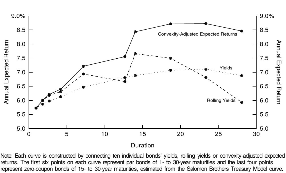
Figure 1 Three Alternative Expected Return Curves, as of 1 Sep 95
In the section "Basics of Convexity", we define convexity, describe how it varies across bonds and discuss the relation between volatility and the value of convexity. We then examine convexity's impact on the yield curve shape and on expected returns and explain why we advocate the use of convexity-adjusted expected returns in the evaluation of duration-neutral barbell-bullet trades. Finally, we present historical evidence about convexity's impact on realized long-term bond returns and on the performance of a barbell-bullet trade.
在“凸度基础”一节中,我们定义凸度,描述债券之间凸度的差异,并讨论波动率与凸度价值之间的关系。然后,我们研究凸度对收益率曲线形状和预期回报的影响,并解释为什么我们主张在久期中性的杠铃-子弹交易的评估中使用凸度调整的预期回报。最后,我们给出凸度对实现的长期债券回报和杠铃-子弹交易表现影响的历史证据。
While this report focuses on convexity's impact on the yield curve (and on bond returns), we stress that the convexity bias is not the only determinant of the yield curve shape. Positive bond risk premia tend to offset the negative impact of convexity, making the yield curve slope upward, at least at short durations. Moreover, the market's expectations about future rate changes can make the yield curve take any shape. This report is the fifth part of a series titled Understanding the Yield Curve; earlier reports in this series describe how the market's rate expectations and the required bond risk premia influence the curve shape.
虽然本报告着重于凸度对收益率曲线(以及债券回报)的影响,但我们强调凸度偏差不是收益率曲线形状的唯一决定因素。正的债券风险溢价倾向于抵消凸度的负面影响,使收益率曲线向上倾斜(至少是在短久期端)。此外,市场对未来收益率变化的预期也可以使收益率曲线发生变化。本报告是《理解收益率曲线》系列的第五部分,本系列的早期报告描述了市场的收益率预期和债券风险溢价如何影响曲线形状。
BASICS OF CONVEXITY [1]
凸度基础
What Is Convexity and How Does It Vary Across Treasury Bonds?
什么是凸度,以及如何因债券不同?
Convexity refers to the curvature (nonlinearity) in a bond's price-yield curve. All noncallable bonds exhibit varying degrees of positive convexity. When a price-yield curve is positively convex, a bond's price rises more for a given yield decline than it falls for a similar yield increase. It is often stated that positive convexity can only improve a bond portfolio's performance. Figure 2, which shows the price-yield curve of a 30-year zero, illustrates in what sense this statement is true: A linear approximation of a positively convex curve always lies below the curve. That is, a duration-based approximation of a bond's price change for a given yield change will always understate the bond price. The error is small for small yield changes but large for large yield changes. We can approximate the true price-yield curve much better by adding a quadratic (convexity) term to the linear approximation. Thus, a bond's percentage price change (\(100 * \Delta P / P\)) for a given yield change is: [2]
凸度是指债券价格-收益率曲线中的曲率(非线性部分)。所有非可赎回债券均呈现不同程度的正凸度。当价格-收益率曲线形态呈下凸时,收益率下降带来的债券价格涨幅要大于同等程度收益率增长带来的价格跌幅。正如通常说的,正凸度只能改善债券组合的表现。图2显示了30年期零息债券的价格-收益率曲线,以说明这一说法在何种程度意义上是正确的:下凸曲线的线性近似总是位于曲线之下。也就是说,对于给定的收益率变化,基于久期近似的债券价格变动将总是低于债券实际价格。(上述偏差)对于小的收益率变化,偏差很小;但是对于大的收益率变化,偏差很大。我们可以通过在线性近似中加上二次项(凸度)来更好地逼近真实的价格-收益率曲线。因此,给定收益率变化的债券百分比价格变化(\(100 * \Delta P / P\))为::
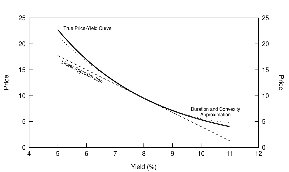
Figure 2 Price-Yield Curve of a 30-Year Zero
where duration = \(-(100/P) * (dP/dy)\), convexity = \(-(100/P) * (d^2P/dy^2)\), \(\Delta y\) is the yield change, and yields are expressed in percentage terms.
其中久期等于\(-(100/P) * (dP/dy)\),凸度等于\(-(100/P) * (d^2P/dy^2)\),\(\Delta y\)是收益率变化,收益率以百分比表示。
In general, the most important determinants of bond convexity are the option features attached to bonds. Bonds with embedded short options often exhibit negative convexity. The negative convexity arises because the borrower's call or prepayment option effectively caps the bond's price appreciation potential when yields decline. However, this report does not analyze bonds with option features. For noncallable bonds, convexity depends on duration and on the dispersion of cash flows (see Appendix A for details).
一般来说,债券凸度最重要的决定因素是债券附带的期权特征。具有嵌入式卖出期权的债券通常呈现负凸度。由于借款人的看涨期权或提前支付期权在收益率下降时有效地限制了债券的价格升值潜力,所以出现了负的凸度。但是,本报告并不分析具有期权特征的债券。对于非可赎回债券,凸度取决于久期和现金流的分散程度(详见附录A)。
Figure 3 shows the convexity of zero-coupon bonds as a function of (modified) duration. Convexity not only increases with duration, but it increases at a rising speed. For zeros, a good rule of thumb is that convexity equals the square of duration (divided by 100).[3] Convexity also increases with the dispersion of cash flows. A barbell portfolio of a short-term zero and a long-term zero has more dispersed cash flows than a duration-matched bullet intermediate-term zero. Of all bonds with the same duration, a zero has the smallest convexity because it has no cash flow dispersion. As discussed in Appendix A, a coupon bonds or a portfolio's convexity can be viewed as the sum of a duration-matched zero's convexity and the additional convexity caused by cash flow dispersion.
图3显示了零息债券的凸度作为(修正)久期的函数。凸度不仅随着久期的推移而增加,而且加速增加。对于零息债券,一个好的经验法则是凸度等于久期的平方(除以100)。随着现金流的分散程度增加,凸度也在增加。短期和长期零息债券的杠铃组合的现金流比久期匹配的中期零息债券的子弹组合更加分散。在具有相同久期的所有债券中,零息债券具有最小的凸度,因为它没有分散的现金流。如附录A所述,付息债券或债券组合的凸度可以被视为久期匹配的零息债券凸度与由现金流分散引起的附加凸度的总和。
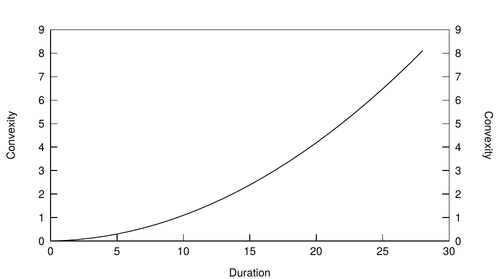
Figure 3 Convexity of Zeros as a Function of Duration
Volatility and the Value of Convexity
波动率和凸度价值
Convexity is valuable because of a basic characteristic of positively convex price-yield curves that we alluded to earlier: A given yield decline raises the bond price more than a yield increase of equal magnitude reduces it. Even if investors know nothing about the direction of rates, they can expect gains to be larger than losses because of the nonlinearity of the price-yield curve. Figure 2 illustrated that convexity has little impact on the bond price if the yield shift is small, but a big impact if the yield shift is large. The more convex the bond and the larger the absolute magnitude of the yield shift, the greater the realized value of convexity is. We do not know in advance how large the realized yield shift will be, but we can measure its expected magnitude with a volatility forecast.[4] If we expect high near-term yield volatility, we expect a high value of convexity.
凸度是有价值的,因为我们早些时候提到的价格-收益率曲线呈现下凸的基本特征:收益率下降提高的债券价格大于收益率增加减少的债券价格。即使投资者对收益率方向一无所知,由于价格-收益率曲线的非线性,他们也可以预期回报将大于损失。图2显示,如果收益率变动小,则凸度对债券价格几乎没有影响;但如果收益率变动较大,则其影响很大。凸度越大并且收益率变动的绝对量越大,实现的凸度价值越大。我们不知道预期实现的收益率变动将会有多大,但是我们可以通过波动率预测来衡量其预期的幅度。如果我们预期近期收益率波动率较大,那么我们预计凸度价值将会很高。
The value of convexity is a nebulous concept; it may be hard for investors to see how higher volatility can increase expected returns. We try to make the concept more concrete and intuitive with the following example. Figure 4 compares the expected value of a 30-year zero in a world of certainty and in a world of uncertainty. In a world of certainty, investors know that a bond's yield will remain unchanged at 8%; thus, there is no volatility and convexity has no value. In the second case, we introduce uncertainty in the simplest possible way: The bond's yield either moves to 10% or to 6% immediately, with equal probability. That is, investors do not know in which direction the rates are moving (on average, they expect no change), but they do know that the rates will shift up or down by 200 basis points. Note that the two possible final bond prices (y = 10%, P = $5.40 and y = 6%, P = $17.00) are higher than those implied by a linear approximation. The expected bond price is an average of the two possible final prices: \(E(P) = 0.5 * \$5.40 + 0.5 * \$17.00 = \$11.20\). This expected price is higher than the price given no yield change (y = 8%, P = $9.50). The $1.70 price difference reflects the expected value of convexity; the bond's expected price is $1.70 higher if volatility is 200 basis points than if volatility is 0 basis points. Thus, higher volatility enhances the (expected) performance of positively convex positions.[5]
凸度价值是一个模糊的概念,投资者可能很难看到波动率会如何提高预期回报。我们尝试通过以下示例使该概念更加具体和直观。图4比较了一个确定性世界和一个不确定性世界的30年期零息债券的预期值。在一个确定的世界中,投资者知道债券的收益率将维持在8%的水平。因此,没有波动性并且凸度没有价值。在第二种情况下,我们以最简单的方式介绍不确定性:债券的收益率跳到10%或6%的概率相等。也就是说,投资者不知道收益率在哪个方向上移动(平均而言,他们预计没有变化),但是他们知道收益率将上升或下降200个基点。请注意,两种可能的最终债券价格(y = 10%, P = $5.40 并且 y = 6%, P = $17.00)高于线性近似隐含的价格。预期债券价格是两种可能的最终价格的平均值:\(E(P) = 0.5 * \$5.40 + 0.5 * \$17.00 = \$11.20\)。这个预期价格高于收益率没有变化的价格(y = 8%, P = $9.50)。1.70的价格差异反映了凸度价值的预期;波动为200个基点时,债券的预期价格比波动为0个基点时高1.70。因此,较高的波动性增强了正凸度头寸的(预期)表现。
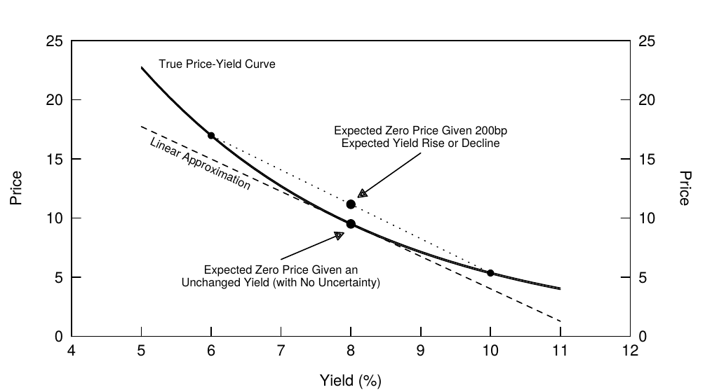
Figure 4 Value of Convexity in the Price-Yield Curve of a 30-Year Zero
The impact of volatility is very clear in the spread behavior between positively and negatively convex bonds (noncallable government bonds versus callable bonds or mortgage-backed securities). It is more subtle in the spread behavior within the government bond market where all bonds exhibit positive convexity. When volatility is high, the yield curve tends to be more humped and is more likely to be inverted at the long end, widening the spreads between duration-matched barbells and bullets and between duration-matched coupon bonds and zeros.
波动率对正-负凸度债券(非可赎回的政府债券与可赎回债券或抵押贷款支持证券)之间利差的影响非常明确。波动率对政府债券市场利差的影响更为微妙,因为所有债券均呈现正凸度。当波动率高时,收益率曲线往往更加弯曲,并且更有可能在长端发生倒挂,扩大久期匹配的杠铃组合和子弹组合之间以及久期匹配的付息债券和零息债券之间的利差。
CONVEXITY, YIELD CURVE AND EXPECTED RETURNS
凸度,收益率曲线与预期回报
Convexity Bias: The Impact of Convexity on the Curve Shape
凸度偏差:凸度对曲线形状的影响
We have demonstrated that positive convexity is a valuable property for a fixed-income asset and that different-maturity bonds exhibit large convexity differences. Now we will show that these convexity differences give rise to offsetting yield differences across maturities. Investors tend to demand less yield for more convex positions because they have the prospect of enhancing their returns as a result of convexity. In particular, Figure 3 showed that long-term bonds exhibit very high convexity. Because of their high convexity, these bonds can offer lower yields than a short-term bond and still offer the same near-term expected returns.
我们已经证明,正的凸度对固定收益资产来说非常有价值,不同期限债券的凸度呈现出巨大差异。现在我们将说明这些凸度差异将会抵消不同期限债券之间的的收益率差异。投资者倾向于要求较低的收益率来获得更多的凸度,因为他们希望通过凸度来提高回报。特别地,图3显示长期债券表现出非常高的凸度。由于较高的凸度,这些债券可以提供比短期债券更低的收益率,并且仍然提供相同的近期预期回报。
We isolate the impact of convexity on the yield curve shape, or the convexity bias[6], by presenting a hypothetical situation where the other influences on the curve shape are neutral. Specifically, we assume that all bonds have the same expected return (8%) and that the market expects the short-term rates to remain at the current (8%) level, and we examine the behavior of the spot curve and the curve of one-year forward rates. With no bond risk premia and no expected rate changes, one might expect these curves to be horizontal at 8%. Instead, Figure 5 shows that they slope down at an increasing pace because lower yields are needed to offset the convexity advantage of long-duration bonds (and thus to equate the near-term expected returns across bonds). Note the symmetry between the curve shapes in Figures 3 and 5.
我们假定其他因素对曲线形状的影响是中性的,以分离凸度对收益率曲线形状的影响(或凸度偏差)。具体来说,我们假设所有债券具有相同的预期回报(8%),市场预期短期收益率将保持在当前(8%)水平,我们研究即期收益率曲线和1年期远期收益率曲线的行为。没有债券风险溢价,没有预期收益率变化,人们可能预期这些曲线在8%上保持水平形状。相反,图5显示曲线加速下降,因为需要较低的收益率来抵消长期债券的凸度优势(并因此使债券的近期预期回报相等)。注意图3和图5中曲线形状之间的对称性。
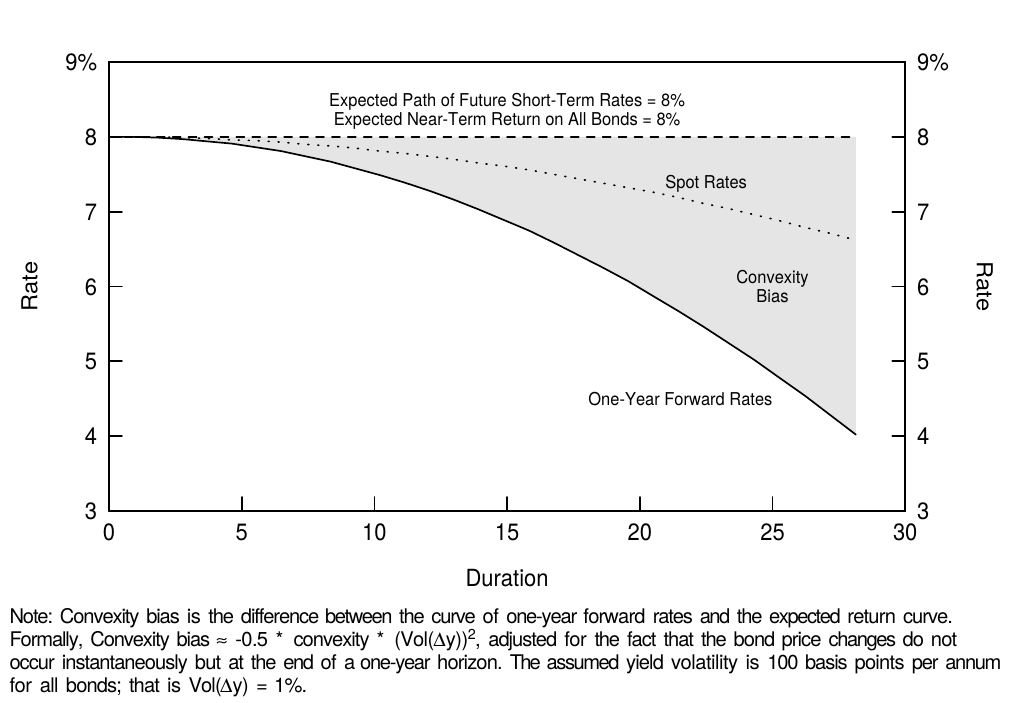
Figure 5 Pure Impact of Convexity on the Yield Curve Shape
Where did the numbers in Figure 5 come from? Unlike the real world, where the spot rates are the easiest to observe, in this example, we take the expected returns as given and work our way back to forward rates and then to spot rates. Given our assumption that the market has no directional views about the yield curve, each zero earns the near-term expected return from the rolling yield[7] and from convexity:[8]
图5中的数字来自哪里?现实世界中即期收益率是最容易观察到的,与此不同,在这个例子中我们假定已知预期回报,并以我们的方式推算远期收益率,然后进一步得到即期收益率。鉴于我们的假设,市场对收益率曲线没有方向性的看法,每个零息债券都能从滚动收益率和凸度中获得近期预期回报:
where value of convexity \(\approx 0.5 * convexity * (Vol(\Delta y))^2\).
其中凸度价值约等于\(0.5 * convexity * (Vol(\Delta y))^2\)。
Using our assumption that all bonds have convexity-adjusted expected return of 8% and using some volatility assumption (which determines the value of convexity), we can back out the rolling yields for various-maturity zeros from Equation (2). Our volatility assumption of 100 basis points means roughly that we expect all rates to move 100 basis points (up or down) from their current level over the next year. For example, if the convexity of a long zero is 2.25 (see footnote 3), the value of convexity is approximately \(0.5 * 2.25 * 1^2 = 1.125\%\). The zero's rolling yield is 6.875% but its annualized near-term expected return is 8%, by assumption. For coupon bonds, which have smaller convexities, the value of convexity is much smaller. The final step in constructing Figure 5 is to compute the spot curve from the curve of one-year forward rates (the rolling yield curve).
基于我们的假设,所有债券的凸度调整预期回报为8%,并使用一些波动率假设(决定凸度价值),我们可以从方程(2)中算出各期限零息债券的滚动收益率。我们的100个基点的波动率假设大概意味着我们预计所有收益率都会从今年的当前水平变化100个基点(上涨或者下降)。例如,如果长期零息债券的凸度为2.25(见注3),凸度价值约为\(0.5 * 2.25 * 1^2 = 1.125\%\)。零息债券的滚动收益率为6.875%,但其年化近期预期回报为8%。对于具有较小凸度的付息债券,凸度价值要小得多。构建图5的最后一步是从1年期远期收益率曲线(即滚动收益率曲线)计算即期收益率曲线。
Convexity bias is simply the inverse of the value of convexity, or \(0.5 * convexity * (Vol(\Delta y))^2\). Figure 5 shows that the convexity bias, by itself, tends to make the yield curve inverted, especially at long durations. However, actual yield curves rarely invert as they do in this hypothetical example, in which we assumed, in particular, that all bonds across the curve have the same near-term expected return and the same basis-point yield volatility. We now relax each of these two assumptions, one at a time. First, convexity is not the only influence on the curve shape. The typical historical yield curve shape is upward sloping, probably reflecting positive bond risk premia (the fact that investors require higher expected returns for long-term bonds than for short-term bonds). At the front end of the curve, the convexity bias is so small that it does not offset the impact of positive bond risk premia. At the long end, the convexity bias can be so large that the yield curve becomes inverted in spite of positive risk premia. Figure 6 shows that in the presence of positive risk premia, convexity bias tends to make the yield curve humped rather than inverted. In this figure, we use historical average returns of various maturity subsectors to proxy for expected returns.
简单讲,凸度偏差是凸度价值的倒数,或者\(0.5 * convexity * (Vol(\Delta y))^2\)。图5显示,凸度偏差本身倾向于使收益率曲线倒挂,特别是在长久期端。然而,实际上收益率曲线很少像这个假设的例子一样出现倒挂,这个例子中我们假设所有期限上的债券都具有相同的近期预期回报并且有相同的基点收益率波动率。我们现在逐个放松这两个假设。首先,凸度不是对曲线形状的唯一影响。典型的收益率曲线形状向上倾斜,可能反映了正的债券风险溢价(相对于短期债券,投资者对长期债券要求更高的预期回报)。在曲线的前端,凸度偏差很小,不能抵消正的债券风险溢价的影响。在曲线长端,尽管有正的风险溢价,但是凸度偏差可能会很大以至于收益率曲线倒挂。图6显示,在存在正的风险溢价的情况下,凸度偏差倾向于使收益率曲线呈现弯曲而不是倒挂。在这个图中,我们使用不同期限的历史平均回报来代表预期回报。
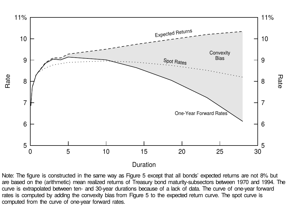
Figure 6 Impact of Convexity with Positive Bond Risk Premia
As explained earlier, the value of convexity increases with yield volatility. Thus far we have assumed that yield volatility is equally high across the curve. Figure 7 shows that historically, the term structure of volatility has often been inverted —— long-term rates have been less volatile than short-term rates. Therefore, the value of convexity does not increase quite as a square of duration even though convexity itself does. However, the value of convexity does increase quite quickly with duration even when the volatility term structure is taken into account; its inversion only dampens the rate of increase (see Figure 8).
如前所述,凸度价值随着收益率的波动率而增加。到目前为止,我们假设收益率波动率在整个曲线上同样高。图7显示,从历史上看,波动率的期限结构往往倒挂,长期收益率的波动幅度低于短期收益率。因此,凸度价值不会像凸度本身一样依久期的平方增大。然而,即使考虑到波动率期限结构,凸度价值确实随着久期的增加而增加;波动率的倒挂只会抑制增加程度(见图8)。
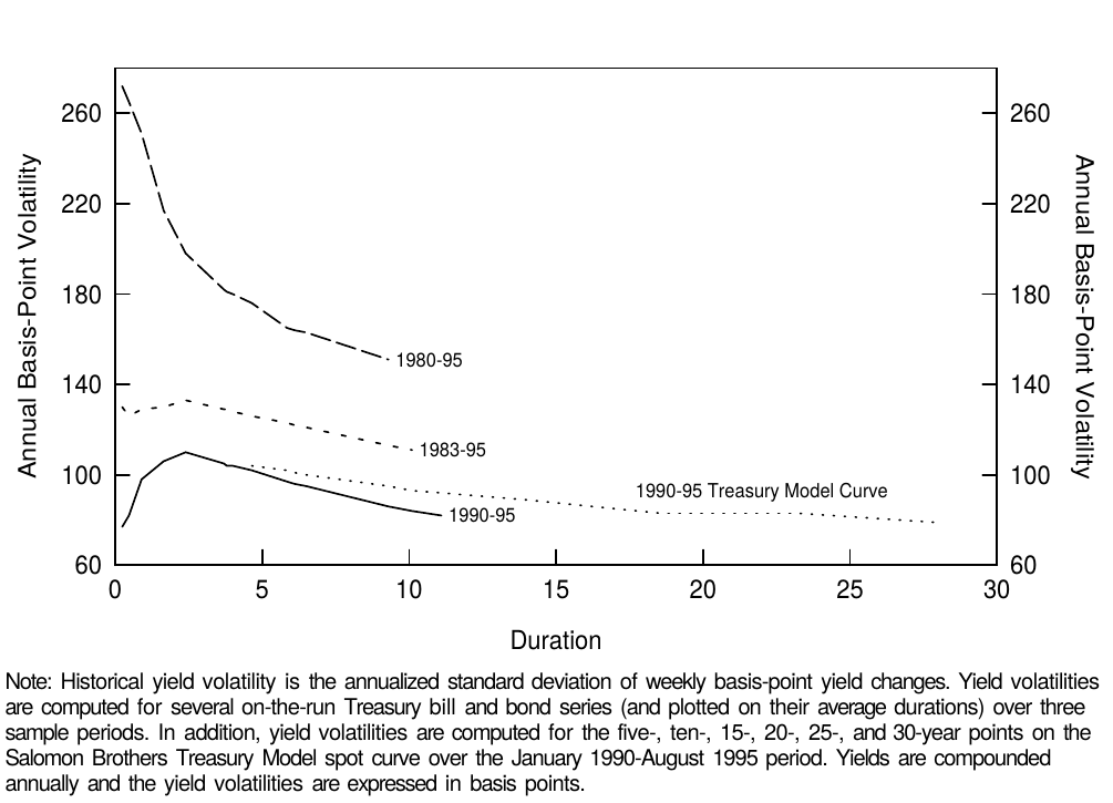
Figure 7 Historical Term Structure of (Basis-Point) Yield Volatility
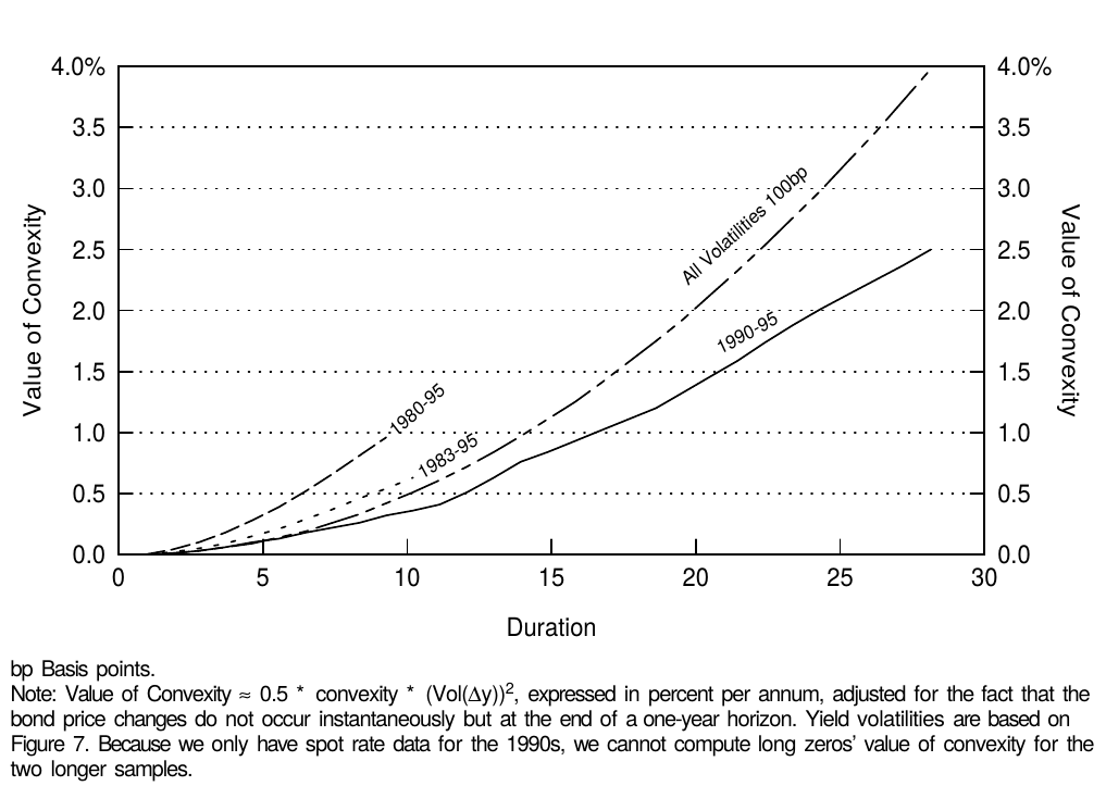
Figure 8 Value of Convexity Given Various Volatility Structures
The levels and shapes of the volatility term structures are very different in Figure 7, depending on the sample period. In the 1980s —— and especially at the beginning of the decade —— yield volatilities were very high and the term structure of volatility was inverted. In the 1990s, volatilities have been lower and the term structure of volatility has been flat or humped. It is difficult to choose the appropriate sample period for computing the yield volatility and Figure 8 shows that this choice will have a significant impact on the estimated value of convexity. Our view is that the relevant choice is between the 1983-95 and the 1990-95 sample periods because we do not expect to see again the volatility levels experienced in 1979-82 —— at least not without clear warning signs. This period coincided with a different monetary policy regime in which the Federal Reserve targeted the money supply and tolerated much higher yield volatility than after October 1982.[9]
图7中,波动率期限结构的水平和形状因样本周期而非常不同。1980年代,特别是初期,收益率的波动率非常高,波动率期限结构倒挂。在1990年代,波动率一直较低,波动率期限结构是平坦或弯曲的。很难选择合适的样本周期计算收益率的波动率,并且图8表明这种选择对凸度价值的估计有重要影响。我们认为合适的选择是在1983-95年和1990-95年期间,因为我们不期望再次看到1979-82年的波动率水平,至少没有明确的警告。这一时期恰好与不同的货币政策制度相联系,美联储盯住货币供应量,容忍收益率波动幅度高于1982年10月以后的水平。
Instead of sample-specific historical volatilities, we could use implied volatilities from current option prices (based on the cap-curve, options on various futures contracts, OTC options on individual on-the-run bonds) to compute the (expected) value of convexity. The main reason that we have not done this is that such implied volatilities are not available for all maturities. In addition, it is not clear from empirical evidence that implied volatilities predict future yield volatilities any better than historical volatilities do.
其实,我们可以使用当前期权价格的隐含波动率(根据cap曲线、各种期货合约的期权、特定债券的OTC期权)来计算(预期)凸度价值,而不是特定样本期的历史波动率。我们没有这样做的主要原因是并不是所有期限都存在这种隐含波动率。此外,从实证证据可以看出,隐含波动率预测未来收益率波动率未必比历史波动率更好。
In Appendix B, we describe the various volatility measures used in this report and discuss the relations between them. In particular, we emphasize that the option prices are typically quoted in relative yield volatilities (\(Vol(\Delta y / y)\)) rather than in the basis-point volatilities (\(Vol(\Delta y)\)) that we use. For example, a 13% implied volatility quote has to be multiplied by the yield level, say 7%, to get the basis-point volatility (91 basis points = 0.91% = 13% * 7%).
在附录B中,我们描述了本报告中使用的各种波动率估计方法,并讨论了它们之间的关系。特别是,我们强调期权价格通常针对相对收益率波动率(\(Vol(\Delta y / y)\)),而不是我们使用的基点波动率(\(Vol(\Delta y)\))。例如,13%的隐含波动率必须乘以收益率水平,如7%,以获得基点波动率(91基点 = 0.91% = 13% * 7%)。
The Impact of Convexity on Expected Bond Returns
凸度对债券预期回报的影响
Figure 8 shows that positive convexity can be quite valuable, especially in a high-volatility environment. However, yield-based measures of expected bond return assign no value to convexity. For example, the rolling yield is a bond's holding-period return given one scenario (an unchanged yield curve), essentially assuming no rate uncertainty. Because volatility can only be positive, the rolling yield is a downward-biased measure of expected return for bonds with positive convexity.[10] Fortunately, it is possible to add the impact of rate uncertainty (the expected value of convexity) to rolling yields. Equation (2) showed that if the base case expectation is an unchanged yield curve, a bond's near-term expected return is simply the sum of the rolling yield and the value of convexity.[11] This relation holds approximately for coupon bonds as well as for zeros.
图8显示,正凸度可以是非常有价值的,特别是在高波动率环境中。然而,基于收益率的债券预期回报度量不认为凸度有任何价值。例如,滚动收益率是给定一种情况(不变收益率曲线)的债券持有期回报,基本上假定没有收益率不确定性。因为波动率只能是正数,所以滚动收益率是对具有正凸度债券的预期回报的下偏度量。幸运的是,可以对滚动收益率添加收益率不确定性(凸度价值的预期)的影响。方程式(2)表明,如果基本情况是期望收益率曲线不变,则债券的近期预期回报只是滚动收益率与凸度价值之和。这种近似关系适用于付息债券以及零息债券。
In Figure 9, we calculate three expected return measures (yield, rolling yield, convexity-adjusted expected return) and the value of convexity on September 1, 1995 for six Treasury par bonds and four long-duration zeros (estimated from the Salomon Brothers Treasury Model curve which represents off-the-run bonds). In addition, we describe two barbell positions that can be compared with duration-matched bullets. Figure 1 showed graphically the three alternative expected return curves as a function of duration.
在图9中,我们计算了1995年9月1日的六个国债和四个长期零息债券的三种预期回报度量(到期收益率、滚动收益率、凸度调整预期回报)和凸度价值(从 Salomon Brothers 国债模型曲线估计,代表不活跃的债券)。此外,我们描述了两个杠铃组合,并与久期匹配的子弹组合进行比较。图1显示了三种预期回报曲线作为久期的函数。
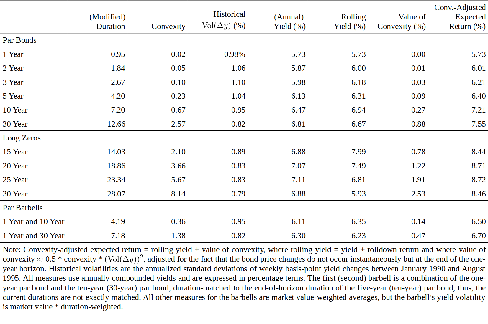
Figure 9 Expected One-Year Returns on Various Bonds as of 1 Sep 95
We use maturity-specific historical volatilities from the 1990-95 period to proxy for expected volatility, and we use a one-year horizon. These choices give one illustration of the ideas developed in this report; we stress that it is possible to use other volatility measures or other horizon. In particular, Figure 7 shows that the volatility estimates would be much higher if we extended our sample period to the 1980s. (The par bonds' yield volatilities are similar to those of the on-the-run bonds in Figure 7.) For a given yield curve, these higher volatility estimates could more than double the estimated value of convexity and, thus, increase the convexity-adjusted expected returns. Using a one-year horizon makes the notation easier because the value of convexity is expressed in annualized terms as are yields and volatilities. If we used a three-month horizon, all three expected return measures and the value of convexity would be roughly one fourth of the numbers in Figure 9. For example, if a 30-year par bond's convexity is 2.57 and the annual volatility is 82 basis points, the quarterly volatility is approximately 41 basis points (\(82 / \sqrt{4}\)), and the quarterly value of convexity is \(0.5 * 2.57 * 0.41^2 = 0.22\%\) (\(\approx 0.88\% / 4\)), or 22 basis points.
我们使用1990-95年期间的特定期限历史波动率来代替预期波动率,样本周期为1年期。这些选择可以说明本报告中提出的想法;我们强调,可以使用其他波动率估计或其他样本周期。特别是,图7显示,如果我们将样本期延长到1980年代,波动率估计将会更高。(债券的收益率波动率与图7中债券的收益率波动率类似)。对于给定的收益率曲线,这些较高的波动率估计可以将凸度价值的估计值增加一倍以上,从而增加凸度调整预期回报。样本周期使用一年使得标记更容易,因为凸度价值以年化收益率表示,正如收益率和波动率。如果我们使用三个月作为样本周期,所有三个预期回报和凸度价值将大约是图9中数字的四分之一。例如,如果30年期债券的凸度为2.57,年化波动率为82基点,季度波动率约为41个基点(\(82 / \sqrt{4}\)),凸度的季度值为\(0.5 * 2.57 * 0.41^2 = 0.22\%\)(\(\approx 0.88\% / 4\))或22个基点。
Figures 1 and 9 show that the convexity adjustment has little impact at short durations because short-term bonds exhibit little convexity. Even for the longest coupon bond, the annual impact is 88 basis points. In contrast, for the longest zeros, the value of convexity is very large both as an absolute number (253 basis points) and as a proportion of their expected return (30% = 2.53/8.46). More generally, the value of convexity can partly explain the rolling yield curve's typical concave (humped) shape, but even the convexity-adjusted expected return curve inverts after 25 years. The longest-maturity zeros appear to have genuinely low expected returns, perhaps reflecting their liquidity advantage and financing advantage.
图1和图9显示,由于短期债券几乎没有凸度,凸度调整对短久期端的影响不大。即使是期限最长的付息债券,年化影响也只是88个基点。相比之下,对于期限最长的零息债券,凸度价值的绝对数(253个基点)和关于预期回报的比例(30% = 2.53 / 8.46)都非常大。更一般地,凸度价值可以部分地解释滚动收益率曲线典型的上凸形状,即使凸度调整的预期回报曲线在25年后倒挂。最长期限的零息债券似乎具有相当低的预期回报,也许反映了其流动性优势和融资优势。
One advantage of this analysis is that it gives an improved view of the overall reward-risk trade-off in the government bond market. Until the 1970s, fixed-income investors evaluated this reward-risk trade-off by plotting bond yields on their maturities. Eventually investors learned that the rolling yield measures near-term expected return better than yield and that duration measures risk better than maturity.[12] In the mid-1980s, investors became familiar with the concept of convexity (see Literature Guide), although few have incorporated it formally into their expected return measures. However, convexity-adjusted expected returns are even better expected return measures than rolling yields —— and the adjustment is reasonably simple. To move all the way to mean-variance analysis, as advocated by the modern portfolio theory, we should adjust bond durations by their yield volatilities; then, Figure 1 would plot bonds' expected returns on their return volatilities. Of course, convexity-adjusted expected returns are not perfect; for example, if investors can predict yield curve reshapings consistently, they can construct even better expected return measures.
这种分析的一个优点是可以更好地看待政府债券市场的总体回报-风险权衡。直到1970年代,固定收益投资者通过画出债券收益率与期限的关系来评估这种回报-风险权衡。最终投资者意识到,在度量近期预期回报方面使用滚动收益率优于收益率,度量风险方面久期要优于期限。在1980年代中期,投资者熟悉了凸度的概念(参见文献指南),尽管很少有人将其纳入预期回报的度量。然而,凸度调整后的预期回报能比滚动收益率更好的度量预期回报,调整也相当简单。正如现代投资组合理论,一切归结为均值-方差分析,我们应该通过收益率波动率来调整债券久期。那么,图1将绘制债券预期回报关于回报波动率的关系。当然,凸度调整的预期回报并不完美。例如,如果投资者可以一致地预测收益率曲线的形变,他们可以构建更好的预期回报度量。
In addition, our analysis helps investors to interpret varying yield curve shapes, and more directly, it gives them tools to evaluate relative value trades between duration-matched barbells and bullets and between duration-matched coupon bonds and zeros. This is the topic of the next subsection.
此外,我们的分析帮助投资者解释不同的收益率曲线形状,并且更直接地,提供了评估久期匹配的杠铃组合和子弹组合之间以及久期匹配的付息债券组合和零息债券组合之间的相对价值交易的工具。这是下一节的主题。
Applications to Barbell-Bullet Analysis
应用于杠铃-子弹组合分析
A barbell-bullet trade involves the sale of an intermediate bullet bond and the purchase of a barbell portfolio of a short-term bond and a long-term bond. Often the trade is weighted so that it is cash-neutral and duration-neutral; that is, one unit of the intermediate bond is sold, a duration-weighted amount of the long bond is bought and the remaining proceeds from the sale are put into "cash" (a short-term bond that matures at the end of horizon). For simplicity, we will only study such barbells in this report. In Appendix A, we explain that a barbell portfolio has a convexity advantage over a duration-matched bullet because the barbell's duration varies more (inversely) with the yield level. Figure 3 provides another illustration of the convexity difference between barbells and bullets. If we draw a straight line between any two points on the zeros' convexity-duration curve, each point on this line corresponds to a barbell portfolio (with varying weights of the long-term and the short-term zero). The convexity of this barbell is the market-value-weighted average of the component bonds' convexities. Because the connecting straight line always lies above the zeros' convexity-duration curve, the barbell's convexity is always higher than that of a duration-matched bullet. Furthermore, the maximum convexity pick-up for any duration occurs when we connect the shortest and longest zeros.
杠铃-子弹交易涉及卖出中期债券(子弹部分)以及买入短期债券和长期债券投资组合(杠铃部分)。通常,交易通过加权使其保持现金中性和久期中性;即中期债券售出一个单位,相应依久期加权的长期债券被买入,剩余的回报被纳入“现金”(在投资期限结束时到期的短期债券) 。为简单起见,我们只会在本报告中研究上述这样的杠铃组合。在附录A中,我们解释说,相对于久期匹配的子弹组合,杠铃组合的长期债券具有凸度优势,因为杠铃组合的久期关于回报水平变化较大。图3提供了杠铃组合和子弹组合之间凸度差异的另一个说明。如果我们在零息债券的凸度-久期曲线上的任意两个点之间画一条直线,则该线上的每个点对应于一个杠铃组合(长期零息债券和短期零息债券具有的不同权重)。这种杠铃组合的凸度是付息债券凸度的市值加权平均。因为连接直线总是位于零息债券的凸度-久期曲线之上,所以杠铃组合的凸度总是高于久期匹配的子弹组合。此外,当我们连接期限最短和最长的零息债券时,任何久期上可以获得的的最大凸度就会出现。
In a similar way, we can connect any two points in Figure 5 and find that the rolling yield of any barbell is below the rolling yield of a duration-matched bullet. More generally, the rolling yield curve (as well as the yield curve) almost always has a concave shape as a function of duration; that is, the curve increases at a decreasing rate or decreases at an increasing rate. Therefore, a rolling yield disadvantage tends to offset the convexity advantage of a barbell-bullet trade. If an investor wants to evaluate the relative cheapness of a barbell-bullet trade, he needs to compare two numbers, the rolling yield give-up and the convexity pick-up. The advantage of the convexity-adjusted expected return is that it provides a single number to measure the attractiveness of these trades. For example, the ones-30s barbell in Figure 9 has a 71-basis-point rolling yield give-up relative to the ten-year bullet (= 6.23% - 6.94%), but how does this give-up compare with the convexity pick-up (1.38 versus 0.67)? The numbers in the last column show that the barbell still has a 51-basis-point give-up (= 6.70% - 7.21%) when measured in terms of convexity-adjusted expected returns and given our volatility forecasts. Incidentally, the shorter barbell in Figure 9 even picks up rolling yield over the duration-matched five-year bullet; this exceptional situation reflects the convex shape in parts of the rolling yield curve in Figure 1.
以类似的方式,我们可以连接图5中的任何两个点,发现任何杠铃组合的滚动收益率低于久期匹配的子弹组合的滚动收益率。更一般地,滚动收益率曲线(以及收益率曲线)几乎总是作为久期的上凸函数;也就是说,曲线以递减的速度增加或以递增的速度减小。因此,滚动收益率劣势倾向于抵消杠铃-子弹交易的凸度优势。如果投资者想要评估杠铃-子弹交易的相对便宜性,他需要比较两个数字,失去的滚动收益率和获得的凸度。凸度调整的预期回报的优点在于它提供了一个单一的数字来衡量这些交易的吸引力。例如,图9中的1-30年期杠铃组合相对于10年期子弹组合失去了71个基点(= 6.23% - 6.94%)的滚动收益率,但是这要如何与获得的凸度(1.38对0.67)比较?最后一列中的数字表明,依据凸度调整后的预期回报和给定的波动率预测值,杠铃组合仍然失去了51个基点(= 6.70% - 7.21%)。顺便说一句,图9中的较短的杠铃组合甚至相对于久期匹配的五年期子弹组合获得了滚动回报;这种特殊情况反映了图1中滚动收益率曲线中的下凸形状。
The performance of a duration-neutral barbell-bullet trade depends on curve reshaping, on parallel curve shifts and on the initial yields: (1) The trade profits from curve flattening and loses from curve steepening (between the two longer bonds); (2) the trade is constructed to be neutral to small parallel curve shifts, but the barbell profits from large shifts in either direction because of its convexity advantage; and (3) the initial rolling yield give-up is greater the more curved (concave) the yield curve is. Such a shape may be caused by the market's expectations of curve flattening or of high volatility, either of which would generate capital gains for the trade in the future.
久期中性的杠铃-子弹交易的表现取决于曲线形变、曲线平行偏移和初始收益率:(1)曲线变平使交易获得利润,曲线变陡(两个较长期限的债券之间)使交易损失;(2)该交易对小的曲线平行偏移保持中性,但杠铃组合由于其凸度优势可以从任一方向的大幅度变化中获利;(3)失去的初始滚动收益率越大,收益率曲线越弯曲(上凸)。这种形状可能是由于市场对曲线变平或高波动率的预期所致,其中任何一种原因都将为未来的交易带来资本回报。
Typical barbell-bullet trades are more curve flattening trades than convexity trades. The following break-even analysis illustrates this point. Consider the long barbell-bullet trade in Figure 9. It consists of selling a ten-year par bond (rolling yield 6.94%) and buying a barbell of the 30-year par bond (rolling yield 6.67%) and the one-year bond (rolling yield 5.73%), with a one-year investment horizon. Thus, at the end of horizon, the components will be a nine-year bond, a 29-year bond and cash. The constraints that the trade is duration-neutral and cash-neutral require weights 0.53 and 0.47 for the long bond and the short bond. Given the duration-neutral weighting of the barbell, the rolling yield give-up is 71 basis points (= 0.53 * 6.67% + 0.47 * 5.73% - 6.94%). We isolate the flattening and convexity effects in the trade by asking two questions:
典型的杠铃-子弹交易更多的是做平曲线,而不是凸度交易。以下盈亏平衡分析显示了这一点。考虑图9中的做多杠铃-子弹交易。卖空10年期债券(滚动收益率6.94%),并购买30年期债券(滚动收益率6.67%)和1年期债券(滚动收益率5.73%)的杠铃组合,投资期一年。因此,在投资期结束时,组合构成将是一个9年期债券,一个29年期债券和现金。久期中性和现金中性的限制要求长期债券和短期债券的权重分别为0.53和0.47。给定杠铃组合的久期中性权重,失去的滚动收益率为71个基点(= 0.53 * 6.67% + 0.47 * 5.73% - 6.94%)。我们通过提出两个问题来区分交易中的做平因素和凸度因素。
- How much would the yield spread between tens and 30s (or more exactly, between nines and 29s at the end of horizon) have to narrow to offset this give-up, if no parallel shifts occur?
- 如果曲线没有发生平行偏移,10年期到30年期之间(或更准确地说是期末的9年期和29年期之间)的利差要收窄多少来抵消失去的滚动收益率?
- How large must the parallel shifts be to make the convexity advantage offset this give-up, if no curve reshaping occurs?
- 如果没有曲线形变,平行偏移必须达到多大才能使凸度优势抵消失去的滚动收益率?
A little math shows that the necessary break-even changes are an 11-basis-point spread narrowing (curve flattening) and a 138-basis-point parallel shift. Historical experience suggests that the former event is more plausible than the latter: Over the past 15 years, the tens-30s spread narrowed by at least 11 basis points in a year 30% of the time, while the ten-year yield level shifted by more than 138 basis points in a year only 17% of the time. Thus, it is more likely that a given rolling yield disadvantage is offset via curve flattening than via the barbell's convexity advantage. However, the relative roles of curve-reshaping and convexity vary across different barbell-bullet trades. The reshaping effects are clearly more important at shorter durations (between most coupon bonds), while convexity can be more important at longer durations (between very long zeros). It follows that the time-variation in the rolling yield spread between barbell and bullet coupon bonds —— or in the yield curve curvature below the ten-year duration —— depends more on the market's changing expectations about future curve flattening/steepening than on its changing volatility expectations.
只需一点数学计算,必要的盈亏平衡变化是一个11个基点的利差收窄(曲线变平)和138个基点的平行偏移。历史经验表明,前一事件比后者更可能发生:在过去15年中,有30%的时间内10年期与30年期的利差收窄至少11个基点,而10年期收益率移动138个基点以上只占17%的时间。因此,给定的滚动收益率劣势更可能通过曲线变平抵消,而不是通过杠铃组合的凸度优势。然而,曲线变形和凸度的相对作用在不同的杠铃-子弹交易中有所不同。在短久期债(大多数付息债券)之间,形变效应显然更为重要,而在长久期债(长期零息债券)之间,凸度可能更为重要。因此,杠铃和子弹债券之间的滚动收益率利差或久期低于10年部分的收益率曲线曲率的时变性,更多取决于市场对未来曲线变平/变陡的预期,而不是其变化的波动率预期。
The convexity aspect of the previous example illustrates the similarity between a barbell-bullet trade and a purchase of a long option straddle (a purchase of a call and a put with the same strike price and exercise date). Figure 10 shows the almost U-shaped pattern that is familiar from option analysis. The rolling-yield disadvantage corresponds to the long call and put positions' initial cost (premium), which large market movements in either direction would offset. The trade would only be profitable if the yield level increased or declined by at least 138 basis points, assuming parallel yield shifts. If the yield curve does not move at all from the initial level, the maximum loss (71 basis points) occurs. Of course, Figure 10 ignores the substantial curve-reshaping risk in this trade.[13]
前一个例子凸度方面的分析说明了杠铃-子弹交易与做多跨式期权交易(购买相同执行价格和执行日期的看涨和看跌期权)之间的相似性。图10显示的几乎呈U形的图案相似于对期权的分析。滚动收益率劣势对应于看涨和看跌期权头寸的初始成本,其中任何一个方向上的大变动都将被抵消这一成本。假设收益率平行变动,如果收益率水平上升或下降至少138个基点,那么交易只会是有利可图的。如果收益率曲线根本不发生移动,则发生最大损失(71个基点)。当然,图10忽略了这个交易中的曲线形变风险。
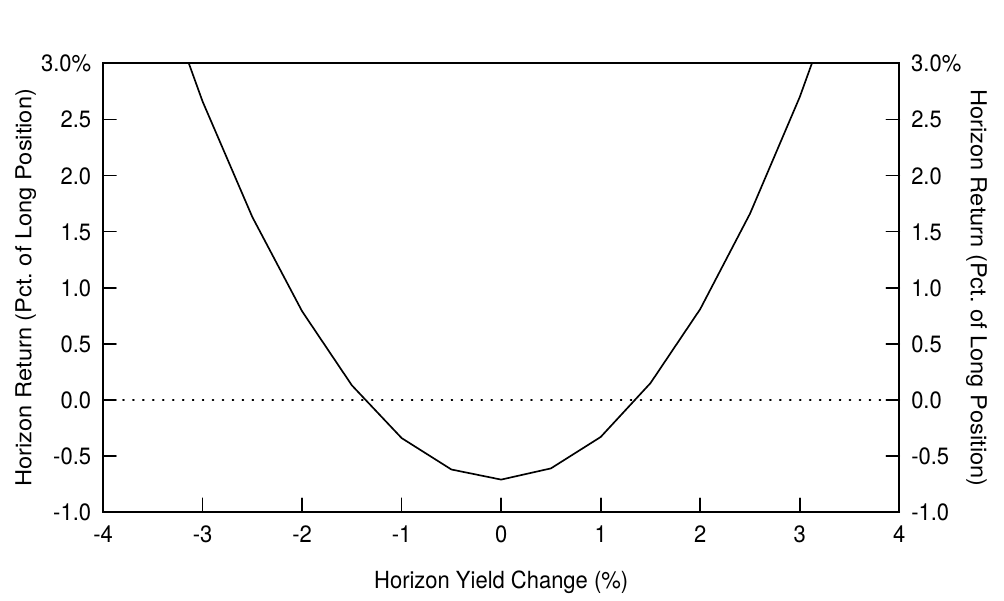
Figure 10 The Payoff Profile of a Barbell-Bullet Trade, Assuming Parallel Yield Shifts
Another way to measure the cheapness of the barbell-bullet trade is to compute its implied yield volatility and compare it with the implied volatility in option markets. We can back out an implied volatility number for each barbell-bullet trade based on the observable rolling yield spread and convexity difference, if we assume that the duration-matched barbell and bullet earn the same expected returns and that the rolling yield spread reflects only the value of convexity —— and no curve-flattening expectations.[14] In that case, high curvature (concavity) in the yield curve and high bullet-barbell rolling yield spreads indicate high implied volatility. In contrast, if the yield curve is a convex function of duration, barbells pick up yield and convexity and the implied volatility is negative —— typically an indication of the market's strong expectations about near-term curve steepening.
衡量杠铃-子弹交易的便宜性的另一种方法是计算其隐含的收益率波动率,并将其与期权市场的隐含波动率进行比较。如果我们假设久期匹配的杠铃组合和子弹组合获得相同的预期回报,并且滚动收益率利差仅反映了凸度价值,没有曲线变平的预期,则可以根据观察到的滚动收益率利差和凸度差异计算出杠铃-子弹交易的隐含波动率。在这种情况下,收益率曲线的高曲率(上凸)和子弹-杠铃组合的高滚动收益率利差表示高的隐含波动率。相比之下,如果收益率曲线是久期的下凸函数,杠铃组合会获得收益率和凸度,并且隐含波动率为负值,这通常表明市场对近期曲线变陡的强烈预期。
HISTORICAL EVIDENCE ABOUT CONVEXITY AND BOND RETURNS
凸度与债券回报的历史依据
The intuition behind convexity-adjusted expected returns is that if investors care about expected return rather than yield, they will rationally accept lower yields and rolling yields from more convex bonds. In this sense, convexity is priced: It influences bond yields. However, a more subtle question is whether convexity also influences expected returns that are not directly observable. It is possible that the rolling yield disadvantage exactly offsets convexity advantage so that two bond positions with the same duration but different convexities have the same near-term expected return. It is also possible that convexity is such a desirable characteristic —— because of the insurance-type payoff pattern —— that the market (investors in the aggregate) accepts lower expected returns for more convex bonds. Finally, it is possible that current-income seekers dominate the marketplace, leading to a price premium (lower expected returns) for higher-yielding, less convex bonds. The jury is still out on this question. The evidence from historical bond returns that we present below suggests that more convex positions earn somewhat lower returns in the long run than less convex positions.
凸度调整预期回报背后的直觉是,如果投资者关心预期回报而不是收益率,那么他们将合理地接受凸度更大而收益率和滚动收益率较低的债券。在这个意义上,凸度通过影响债券收益率而被定价。然而,一个更微妙的问题是凸度是否也影响不可直接观察到的预期回报。滚动收益率劣势可能完全抵消凸度优势,使得具有相同久期但不同凸度的两个债券头寸具有相同的近期预期回报。由于保险型回报模式,凸度是有吸引力的特点,即市场(总体投资者)因为债券较大的凸度而接受期较低的预期回报。最后,追逐眼下回报的投资者有可能在市场上占主导地位,导致了高回报、小凸度债券的价格溢价(较低的预期回报)。这个问题还没有定论。下文中来自历史债券回报的证据表明,凸度较大的头寸从长期来看回报略低于凸度较小的头寸。
In this final section, we examine the historical performance of a long-term bond position and of a wide barbell-bullet position between January 1980 and December 1994, focusing on the impact of convexity on realized returns. The first strategy involves always investing in the on-the-run 30-year Treasury bond; this strategy is long convexity by holding a long-duration bond. The second strategy involves rolling over a fives-thirties flattening trade each month. Specifically, we sell short the on-the-run five-year Treasury bond each month and buy a barbell of the 30-year bond and one-month bill. The trade is duration-matched to horizon; that is, the weight of the 30-year bond in the barbell is such that the barbell and the bullet have the same expected duration at the end of the month. A little algebra shows that the weight is the ratio of the five-year bond's duration to the 30-year bond's duration (at horizon). Although the trade is cash-neutral and duration-neutral, it is long convexity because a barbell is more convex than a bullet.
在本篇最后一节中,我们研究了1980年1月至1994年12月期间的长期债券头寸以及杠铃-子弹组合的历史表现,重点是凸度对实现回报的影响。第一个策略总是投资于当期(活跃的)30年期的国债;这种策略通过持有长期债券而做多凸度。第二个策略涉及到在5年期与30年期债券之间反复做月度做平交易。具体来说,我们每月做空五年期国债,并做多30年期债券和一个月期国库券。久期和投资期限匹配,也就是说,30年期债券的权重使得杠铃组合和子弹组合在月底有相同的预期久期。简单计算表明,权重是五年期债券久期与30年期债券久期的比例。虽然交易是现金中性和久期中性的,但它是做多凸度的,因为杠铃组合比子弹组合的凸度更大。
We first show some summary statistics of various bond positions in Figure 11 but focus on the last two columns. The bullet has roughly a 100-basis-point higher average return and average yield than the duration-matched barbell.[15] Thus, the barbell's convexity pick-up (0.69 versus 0.19) and the impact of yield curve reshaping do not offset its initial yield give-up. However, the barbell does have clearly lower return volatility than the bullet, reflecting the lower yield volatility of the 30-year bond than the five-year bond.
我们首先在图11中显示各种债券头寸的一些汇总统计数据,但重点在最后两列。子弹组合比久期匹配的杠铃组合多大约100个基点的平均收益率和平均收益率。因此,杠铃组合获得的凸度(0.69对0.19)和收益率曲线形变的影响并不能抵消其损失的初始收益率。然而,杠铃组合的回报波动率明显低于子弹组合,这反映了30年期债券的收益率波动率比五年期债券低。
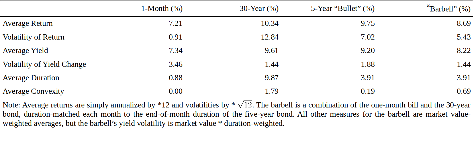
Figure 11 Description of Various On-the-Run Bond Positions, 1980-94
We can decompose any bond's holding-period return into four parts: the yield impact; the duration impact; the convexity impact; and a residual term. Recall from Equation (1) that duration and convexity effects can approximate a bond's instantaneous return well. Over time, a bond also earns some income from coupons or from price accrual; we estimate this income from a bond's yield. Thus, we approximate a bond's holding-period return by Equation (3).[16] The difference between the actual return and its three-term approximation is the residual term; if the approximation is good, the residual should be relatively small. We split the 30-year bond's monthly returns to four components and describe the average behavior and volatility of each component in the top panel of Figure 12.[17]
我们可以将债券的持有期回报分解为四个部分:收益率影响、久期影响、凸度影响和误差项。从等式(1)回顾,久期和凸度因素可以近似债券的即时回报。随着时间的推移,债券还可以从票息或价格中获得一些收入;我们从债券的收益率中估算这笔收入。因此,我们通过公式(3)近似债券的持有期回报。实际回报与其三项近似值之间的差额是误差项;如果近似值较好,则误差项应相对较小。我们将30年期债券的月度回报分为四个组成部分,并在图12中描述了各个成分的平均行为和波动率。
The return volatility numbers in the top panel of Figure 12 show that in any given month, the duration impact largely drives the long bond's return —— it is the source behind 99% of the monthly return fluctuations. However, yield increases and decreases tend to offset each other over time, having little impact on long-term average returns.[18] Over our 15-year sample period, the long bond's average return reflects more the average yield (91%) and less the convexity (14%) and duration (-5%) effects. The residual term has a small mean and volatility, indicating that the approximation in Equation (3) works well. Subperiod analysis shows that over three-year horizons, the duration effect can still have a significant positive or negative impact —— the 1983-85 and 1989-91 subperiods were clearly bull markets and the three other subperiods were bear markets. In contrast, the yield and convexity effects are always positive (by construction). The convexity impact was largest in the early 1980s when yield volatility was very high. During the whole sample, the annualized convexity impact was 148 basis points. In the 1990s, it was about half of that.
图12顶部的回报波动率数据显示,在任何一个月,久期很大程度上影响了长期债券的回报,这是每月回报波动99%的来源。但是,随着时间的推移,收益率的增加和减少往往相互抵消,对长期平均回报影响不大。在15年的样本期,长期债券的平均回报更多反映了平均收益率(91%)的影响,其次是凸度(14%),再次是久期(-5%)。误差项具有小的均值和波动率,表明等式(3)中的近似程度很好。子时段分析显示,三年内久期仍然可以产生显着的正面或负面影响,1983-85年和1989-91年显然是牛市,另外三个子时段是熊市。相比之下,收益率和凸度因素总是正的。1980年代初,当收益率波动率很大时,凸度的影响最大。在整个样本中,年化凸度影响为148个基点,而在1990年代,大约只是一半。
Similarly, we can split the five-year bullet's and the duration-matched barbell's monthly returns into four components based on Equation (3). The lower panel of Figure 12 describes the average behavior and volatility of their difference, which can be viewed as a duration-matched and cash-neutral barbell-bullet trade. Again, the volatility numbers show that most of the monthly fluctuations (99%) come from the duration impact. The trade is duration-neutral; thus, the duration impact refers to the capital gains or losses caused by curve reshaping. That is, although \(Dur_{Barbell} = Dur_{Bullet}\), the duration impacts of the barbell and the bullet differ unless the yield changes are parallel (\(-Dur_{Barbell} * \Delta y_{Barbell} \neq -Dur_{Bullet} * \Delta y_{Bullet}\)). Over the whole sample, these effects tend to cancel out, and the average return depends largely (90%) on initial yields. The barbell has a 105-basis-point lower average annual return than the bullet, mainly because of its yield disadvantage (-95 basis points) and partly due to losses caused by the curve steepening (-36 basis points); these are only partly offset by the barbell's convexity advantage (30 basis points). In four out of five subperiods, the bullet outperformed the barbell, suggesting that a barbell's convexity advantage is rarely sufficient to offset the negative carry over a multiyear period.[19] In addition, the impact of curve-reshaping is larger, in absolute magnitude, than the convexity impact in each subperiod. Again, the residual has a small mean and volatility; thus, the approximation in Equation (3) appears to work well.
同样地,我们可以根据公式(3)将五年期子弹组合和久期匹配的杠铃组合的月回报分为四个成分。图12的下半部分显示了它们差异的平均行为和波动性,可以看作是久期匹配和现金中性的杠铃-子弹交易。同样,波动率数据显示,大部分(99%)月度波动来自久期的影响。交易是久期中性的,因此,久期的影响是指由曲线变形引起的资本损益。也就是说,尽管\(Dur_{Barbell} = Dur_{Bullet}\),杠铃组合和子弹组合的久期影响也是不同的,除非收益率变化是平行的(\(-Dur_{Barbell} * \Delta y_{Barbell} \neq -Dur_{Bullet} * \Delta y_{Bullet}\))。在整个样本中,这些影响趋于抵消,平均回报主要取决于初始收益率(90%)。杠铃组合的平均年化回报比子弹组合低105个基点,主要是由于其收益率劣势(-95个基点),部分原因是由于曲线变陡造成的损失(-36个基点),杠铃组合的凸度优势仅可以抵消部分(30个基点)。五分之四的时段内,子弹组合的表现优于杠铃组合,这表明杠铃组合的凸度优势在多个时段内不足以抵消负的Carry。此外,从绝对值的角度看,在每个子时段内曲线变形的影响大于凸度的影响。残差具有小的平均值和波动率,因此等式(3)中的近似良好。
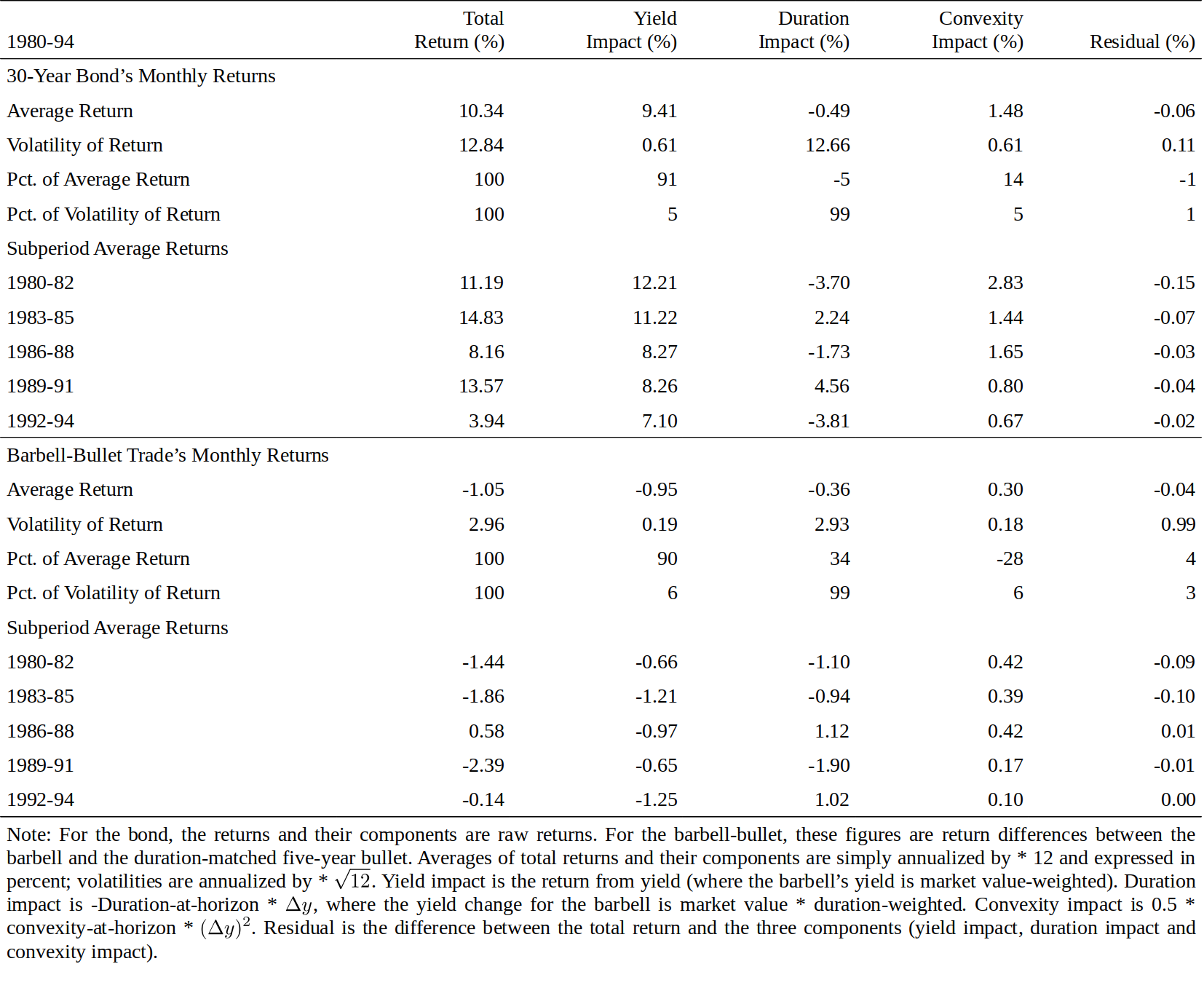
Figure 12 Decomposing Returns to Yield, Duration and Convexity Effects
Figure 12 describes the impact of convexity, and two other effects, on realized bond returns. While characterization of past returns is sometimes useful, most investors are more interested in the future impact of convexity. If volatility and convexity were constant, we could use the historical average convexity impact to proxy for the expected value of convexity. However, volatility and convexity vary over time. Figure 13 shows the behavior of convexity, the rolling 20-day historical volatility and the (expected) value of convexity of the 30-year bond between 1980 and 1994. (Recent historical volatility is often used as an estimate for near-term future volatility.) Convexity has increased as yields declined, but the volatility level has declined even more except for spikes after the 1987 stock market crash and after the Fed's tightening in spring 1994. In the early 1980s, convexity was worth several hundred basis points for the 30-year bond —— while more recently, the value of convexity has rarely exceeded 100 basis points. Such variation implies that any estimates of the value of convexity are as good as the underlying estimates of future volatility. Therefore, when computing convexity-adjusted expected returns, investors should use the information in the current yield curve combined with their best forecasts of the near-term yield volatility.
图12描述了凸度以及另外两个影响对实现债券回报的影响。虽然过去回报的表征有时是有用的,但大多数投资者对未来的凸度影响更感兴趣。如果波动性和凸度不变,我们可以使用历史平均凸度影响来代表预期的凸度值。然而,波动性和凸度随时间而变化。图13显示了1980年至1994年期间的凸度、20天滚动历史波动率和30年期债券凸度(预期)的趋势。(近期历史波动率通常用作近期未来波动率的估计值。)随着收益率的下降凸度有所增加,但1987年以来股市暴跌之后以及美联储在1994年春季收紧财政之后,波动幅度也有所下降。1980年代初期,对于30年期债券来说,凸度价值几百个基点,而近期凸度的价值很少超过100个基点。这种变化意味着对凸度价值的任何估计与未来波动率的基本估计一样好。因此,当计算凸度调整后的预期回报时,投资者应使用当前收益率曲线中的信息及其对近期收益率波动率的最佳预测。
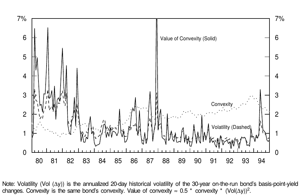
Figure 13 Convexity and Volatility of the 30-Year Bond Over Time
APPENDIX A. HOW DOES CONVEXITY VARY ACROSS NONCALLABLE TREASURY BONDS?
附录 A:非可赎回国债的凸度变化
For bonds with known cash flows, convexity depends on the bond's duration and on the dispersion of the bond's cash flows. The longer the duration, the higher the convexity (for a given cash flow dispersion), and the more dispersed the cash flows, the higher the convexity (for a given duration). In this subsection, we discuss the algebra and the intuition behind these relations. We begin by analyzing zero-coupon bonds.
对于已知现金流的债券,凸度取决于债券的久期和债券现金流的分布。久期越长,凸度越高(给定现金流分布);现金流越分散,凸度越高(给定久期)。在本小节中,我们讨论这些关系背后的数学和直觉。我们首先分析零息债券。
The price of an n-year zero is
n年期零息债券的价格为
where P is the bond's price, y is its annually compounded yield, expressed in percent, and n is its maturity. Taking the derivative of price with respect to yield reveals that
其中P为债券的价格,y为其年化收益率,以百分比表示,n为其期限。对收益率求导数得出
The second equality holds because \(1/(1+y/100)^n = P / 100\), based on Equation (4). Multiplying both sides of Equation (5) by \((-100/P)\) gives the definition of (modified) duration:
由于\(1/(1+y/100)^n = P / 100\),基于等式(4),所以第二个等式成立。将等式(5)的两边乘以\((-100/P)\),给出(修正)久期的定义:
For zeros, maturity (n) equals Macaulay duration (T). Thus, Equation (6) confirms the familiar relation between modified duration and Macaulay duration: \(Dur = T / (1+y/100)\), given annual compounding.
对于零息债券,期限(n)等于Macaulay久期(T)。因此,等式(6)证实了修正久期和 Macaulay 久期之间的关系:\(Dur = T / (1+y/100)\),给定每年付息一次。
Taking the second derivative of price with respect to yield reveals that,
对价格关于收益率求二阶导数得到,
Multiplying both sides by \((100/P)\) gives the definition of convexity (Cx):
两边同时乘以\((100/P)\),给出凸度(Cx)的定义:
Expressed in terms of Macaulay duration or modified duration, a zero's convexity is \((T^2+T)/[100*(1+y/100)^2]/100\). For long-term bonds —— the square of duration is much larger than duration, thus, the rule of thumb that the convexity of zeros increases as a square of duration divided by 100. For example, for a zero with modified duration of 20 and yield of 8%, convexity is approximately 4.0 (\(=20^2/100 \approx (20^2 + 20/1.08)/100 = 4.8\)).
以 Macaulay 久期或修正久期表示,零息债券的凸度为\((T^2+T)/[100*(1+y/100)^2]/100\)。对于长期债券,久期的平方比久期大得多,因此,零息债券的凸度约等于久期的平方除以100。例如,对于修改久期为20且收益率为8%的零息债券,凸度约为4.0。
The relation between the convexity and duration of zeros, illustrated in Figure 3, is simply a mathematical fact. With Figure 14 we try to offer some intuition as to why long-term bonds have much more nonlinear (convex) price-yield curves than short-term bonds. This figure shows price as a function of yield for various-maturity zeros. All curves are downward sloping but not linear. However large the discounting term \((1+y/100)^n\) is, prices cannot become negative as long as \(y > 0\). Intuitively, high convexity (that is, a large change in the slope of the price-yield curve) is needed to keep bond prices positive if the price-yield curve is initially very steep. Otherwise the linear approximation of the long bond's price-yield curve would hit zero very fast (at a yield of 11% for a 30-year zero in Figure 14 versus at a yield of 43% for a three-year zero).
如图3所示,零息债券的凸度和久期之间的关系是一个简单的数学事实。与图14一样,我们试图提供一些直觉,说明为什么长期债券的价格-收益率曲线比短期债券具有更强的非线性(凸度)。这幅图显示了不同期限零息债券的价格作为收益率的函数。所有曲线都是向下倾斜,但不是线性的。然而,不管贴现项\((1+y/100)^n\)有多大,只要\(y > 0\),价格就不会变为负值。直接上,如果价格-收益率曲线最初很陡,需要大的凸度(即价格-收益率曲线大的斜率变化)来保持债券价格是正的。否则,长期债券的价格-收益率曲线的线性近似将非常快速地达到零(图14中的30年零息债券将在收益率为11%时为零,而三年期零息债券在收益率为43%时为零)。
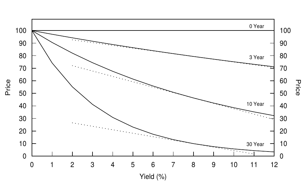
Figure 14 Price-Yield Curves of Zeros with Various Maturities and Their Linear Approximations
For a given duration, convexity increases with the dispersion of cash flows. A barbell portfolio of a short-term zero and a long-term zero has more dispersed cash flows than a duration-matched bullet intermediate-term zero. The bullet, in fact, has no cash flow dispersion. The barbell exhibits more convexity because of the inverse relation between yield level and portfolio duration. A given yield rise reduces the present value of the longer cash flow more than it reduces that of the shorter cash flow, and the decline in the longer cash flow's relative weight shortens the barbell's duration, limiting losses if yields rise further. (Recall that the Macaulay duration of a portfolio is the present-value-weighted average duration of its constituent cash flows.) Of all bonds with the same duration, a zero has the smallest convexity because it has no cash flow dispersion. Thus, its Macaulay duration does not vary with the yield level.
给定久期,凸度随着现金流的分散程度增加。短期和长期零息债券杠铃组合的现金流比久期匹配的中期零息债券子弹组合更分散。事实上,子弹组合的现金流没有分散。由于收益率水平与投资组合久期之间的反比关系,杠铃组合表现出更多的凸度。相对于短期现金流,给定的收益率上涨更会降低长期现金流的现值,而且长期现金流相对权重的下降会缩短杠铃组合的久期,从而限制了收益率进一步上涨时的损失。(回想一下,投资组合的 Macaulay 久期是其组合现金流的现值加权平均久期。)在所有久期相同的债券中,由于没有现金流分散,零息债券的凸度最小。因此,其 Macaulay 久期并不随收益率水平而变化。
In fact, a coupon bond's or a portfolio's convexity can be viewed as a sum of a duration-matched zero's convexity and additional convexity caused by cash flow dispersion. That is, the convexity of a bond portfolio with a Macaulay duration T is:
事实上,付息债券或投资组合的凸度可以看做是一系列久期匹配的零息债券的凸度之和加上由于现金流分散造成的附加凸度。Macaulay 久期为 T 的债券组合的凸度是:
where the first term on the right-hand side equals a duration-matched zero's convexity (see Equation (8)) and "dispersion" is the standard deviation of the maturities of the portfolio's cash flows about their present-value-weighted average (the Macaulay duration).[20]
其中右侧的第一项等于久期匹配的零息债券的凸度(参见等式(8)),并且“Dispersion”是 投资组合现金流的期限关于其现值加权平均(Macaulay 久期)的标准差。
Figure 15 illustrates the convexity difference between a bullet (a 30-year zero) and a duration-matched barbell portfolio of ten-year and 50-year zeros, We use such an extreme example and a hypothetical 50-year bond only to make the difference in the two price-yield curve shapes visually discernible. If the yield curve is flat at 8% and can undergo only parallel yield shifts, the barbell will, at worst, match the bullets performance (if yields stay at 8%) and, at best, outperform the bullet substantially (if yields shift up or down by a large amount). Clearly, high positive convexity is a valuable characteristic. In fact, because it is valuable, the situation in Figure 15 is unrealistic. If the flat curve / parallel shifts assumption were literally true, investors could earn riskless arbitrage profits by being long the barbell and short the bullet. In reality, market prices adjust so that the yield curve is typically concave rather than flat (that is, the barbell has a lower yield than the bullet), and nonparallel shifts such as curve steepening can make the bullet outperform the barbell.
图15显示了子弹组合(30年零)和久期匹配的杠杆组合(10年期和50年期零息债券)之间的凸度差异,我们使用这样一个极端的例子和一个假设的50年期债券使得两个价格-收益率曲线形状的差异在视觉上可辨别。如果收益率水平为8%,并且收益率只能平行变动,那么最坏的情况下杠铃组合的表现会和子弹组合一致(如果收益率保持在8%),而最好的情况是杠铃组合大幅跑赢子弹组合(如果收益率大幅度上升或下降)。显然,凸度大是一个有价值的特征。其实,因为它是有价值的,图15的情况是不切实际的。如果曲线水平并且平行偏移的假设是真实的,投资者可以通过做多杠铃组合做空子弹组合获得无风险的套利利润。实际上,市场价格的调整使得收益率曲线通常是上凸的而不是水平的(杠铃组合比子弹组合的收益率更低),并且曲线非平行的变化(如曲线变陡峭)可以使得子弹组合跑赢杠铃组合。

Figure 15 Price-Yield Curves of a Barbell and a Bullet with the Same Duration (30 Years)
APPENDIX B. RELATIONS BETWEEN VARIOUS VOLATILITY MEASURES
附录 B:不同波动率度量方法间的关系
Equation (1) shows that \(0.5*Cx*(\Delta y)^2\) approximates the impact of convexity on a bond's percentage price changes. Thus, the expected value of convexity \(\approx 0.5*Cx*E(\Delta y)^2\). Now we discuss relations between \(E(\Delta y)^2\) and some volatility measures. The variance of basis-point yield changes is defined as
公式(1)表明,\(0.5 * Cx * (\Delta y)^2\)近似于凸度对债券价格变动百分比的影响。因此,凸度价值的预期约等于\(0.5 * Cx * E(\Delta y)^2\)。现在我们讨论\(E(\Delta y)^2\)与一些波动率度量方法之间的关系。收益率变动的方差定义为
Because yield changes are mostly unpredictable, it is reasonable to assume that \(E(\Delta y) \approx 0\). Therefore, \(Var(\Delta y) \approx E(\Delta y - 0)^2 = E(\Delta y)^2\). The volatility of yield changes (\(Vol(\Delta y)\)) is often measured by standard deviation —— the square root of variance. Thus,
由于收益率变化是不可预测的,因此有理由假设\(E(\Delta y) \approx 0\)。因此,\(Var(\Delta y) \approx E(\Delta y - 0)^2 = E(\Delta y)^2\)。收益率变化的波动率(\(Vol(\Delta y)\))通常是指标准差,即方差的平方根。因此
As long as \(E(\Delta y) \approx 0\), volatility is roughly proportional to the expected absolute magnitude of the yield change, \(E(|\Delta y|)\). Note that it makes sense to assume that \(E(|\Delta y|)\) is positive even when \(E(\Delta y) = 0\). Even if an investor thinks that the current yield curve is the best forecast for next year's yield curve, he can think that the curve is likely to move up or down by, say, 100 basis points from the current level over the next year. In fact, it would be extreme to assume that \(E(|\Delta y|) = 0\); this assumption would imply zero volatility (no rate uncertainty).
只要\(E(\Delta y) \approx 0\),波动率与收益率变化的绝对值期望(\(E(|\Delta y|)\))大致成正比。注意,即使\(E(\Delta y) = 0\),\(E(|\Delta y|)\)也是正的。即使投资者认为目前的收益率曲线是对明年收益率曲线的最佳预测,该曲线在明年也有可能相对于今年水平向上或向下移动100个基点。事实上,假设\(E(|\Delta y|) = 0\)将是极端的,因为这个假设将意味着零波动率(不存在不确定性)。
Next we show that for zero-coupon bonds the value of convexity is proportional to the variance of returns. Both yields and returns are expressed in percent. Short-term fluctuations in bonds' holding-period returns (h) mostly reflect the duration impact (\(-Dur * \Delta y\)) because the yield and convexity impacts are either so stable or so small that they contribute little to the return variance (see Equation (3) and Figure 12). Therefore,
接下来我们说明,零息债券的凸度价值与回报方差成比例。收益率和收益率都以百分比表示。债券持有期回报的短期波动主要反映久期的影响(\(-Dur * \Delta y\)),因为收益率和凸度的影响要么稳定要么很小,所以它们对回报方差贡献不大(见等式(3)和图12)。因此,
The relation \(Cx \approx Dur^2 / 100\) is explained below Equation (8). A comparison of Equations (11) and (12) shows that the value of convexity for zeros is approximately equal to the variance of returns divided by 200. Interestingly, also the difference between an arithmetic mean and a geometric mean is approximately equal to the variance of returns divided by 200.[21] It appears that a duration extension enhances convexity and increases the (arithmetic) expected return, but the ensuing increase in volatility drags down the geometric mean and offsets the convexity advantage.
下面等式(8)说明关系\(Cx \approx Dur^2 / 100\)。方程(11)和(12)的比较表明,零息债券的凸度价值近似等于回报方差除以200。有趣的是,算术平均值和几何平均值之间的差异近似等于回报的方差除以200。看来,增大久期会增加凸度并增加(算术)预期回报,但是随之而来的波动性增加会拖累几何平均值并抵消凸度优势。
Equation (12) illustrates the relation between a bond's return volatility and yield volatility. We finish by stressing the distinction between the volatility of basis-point yield changes \(Vol(\Delta y)\) and the volatility of relative yield changes \(Vol(\Delta y / y)\). The volatility quotes in option markets and in Bloomberg or Yield Book typically refer to \(Vol(\Delta y / y)\), while our analysis focuses on \(Vol(\Delta y)\).
公式(12)说明了债券回报波动率与收益率波动率之间的关系。最后,我们强调基点收益率变动的波动率(\(Vol(\Delta y)\))与相对收益率变动的波动率(\(Vol(\Delta y / y)\))之间的区别。期权市场和彭博或收益率手册中的波动率通常指\(Vol(\Delta y / y)\),而我们的分析则集中在\(Vol(\Delta y)\)上。
In Figure 7, we use the historical basis-point yield volatility to proxy for the expected basis-point yield volatility. Alternatively, we could compute the historical relative yield volatility and multiply it by the current yield level. The latter approach would be appropriate if the relative yield volatility is believed to be constant over time, making the basis-point yield volatility vary one-for-one with the yield level. Empirically, this has not been the case in the United States since 1982 (see footnote 9).
在图7中,我们使用历史基点收益率波动率来代表预期基点收益率波动率。或者,我们可以计算历史相对收益率波动率,并将其乘以当前收益率水平。如果相对收益率波动率被认为是不随时间变化的,后一种方法将比较适当,这使得基点收益率波动率随着回报水平变化。经验上,自1982年以来,美国并非如此(见注9)。
LITERATURE GUIDE
文献指南
On the Basics of Convexity
关于凸度的基本知识
- Garbade, Bond Convexity and its Implications for Immunization, Bankers Trust Co., March 1985.
- Klotz, Convexity of Fixed-Income Securities, Salomon Brothers Inc, October 1985.
- Ho, Strategic Fixed-Income Investment, 1990.
- Diller, "Parametric Analysis of Fixed Income Securities," in Fixed Income Analytics, ed. by Dattatreya, 1991.
- Fabozzi, Bond Markets, Analysis and Strategies, 1993.
- Tuckman, Fixed Income Securities, 1995.
On the Impact of Convexity on the Yield Curve Shape
关于凸度对收益率曲线形状的影响
- Cox, Ingersoll, and Ross, "A Re-examination of Traditional Hypotheses about the Term Structure of Interest Rates," Journal of Finance, 1981.
- Campbell, "A Defense of Traditional Hypotheses about the Term Structure of Interest Rates," Journal of Finance, 1986.
- Diller, "The Yield Surface," in Fixed Income Analytics, ed. by Dattatreya, 1991.
- Litterman, Scheinkman, and Weiss, "Volatility and the Yield Curve," Journal of Fixed Income, 1991.
- Christensen and Sorensen, "Duration, Convexity, and Time Value," Journal of Portfolio Management, 1994.
On the Impact of Convexity in the Context of Multi-Factor Term Structure Models
关于多因子期限结构模型下凸度的影响
- Brown and Schaefer, "Interest Rate Volatility and the Shape of the Term Structure," working paper, London Business School, 1993.
- Gilles, "Forward Rates and Expected Future Short Rates," working paper, Federal Reserve Board, 1994.
On the Empirical Impact of Convexity on Bond Yields and Returns
关于凸度对债券收益率和回报影响的实证分析
- Kahn and Lochoff, "Convexity and Exceptional Return," Journal of Portfolio Management, 1990.
- Lacey and Nawalkha, "Convexity, Risk, and Returns," Journal of Fixed Income, 1993.
This section provides a brief overview of convexity. Readers who are not familiar with this concept may want to read first a text with a more extensive discussion, such as Klotz (1985) or Tuckman (1995).
本小节提供了关于凸度的简要介绍,还不熟悉凸度概念的读者可以先阅读 Klotz(1985)或 Tuckman(1995)的文献 ↩︎Equation (1) is based on a two-term Taylor series expansion of a bond's price as a function of its yield, divided by the price. The Taylor series can be used to approximate the bond price with any desired level of accuracy. A duration-based approximation is based on a one-term Taylor series expansion; it only uses the first derivative of the price function (\(dP/dy\)). The two-term Taylor series expansion also uses the second derivative (\(d^2P/dy^2\)) but ignores higher-order terms. In Equation (1), the word "convexity" is used narrowly for the difference between the two-term approximation and the linear approximation, but the word is sometimes used more broadly for the whole difference between the true price-yield curve and the linear approximation. Given the price-yield curves of Treasury bonds and typical yield volatilities in the Treasury market, the two-term approximation in Equation (1) is quite accurate. As an "eyeball test," we note that Figure 2 shows the most nonlinear price-yield curve among noncallable Treasury bonds and yet, the two-term approximation is visually indistinguishable from the true price-yield curve within a 300-basis-point yield range.
作为收益率函数的债券价格进行二阶 Taylor 级数展开,再除以价格,得到等式(1)。Taylor 级数可以以任何精度近似债券价格。基于久期的近似建立于一阶 Taylor 级数展开;它只使用价格函数的一阶导数(\(dP/dy\))。二阶 Taylor 级数展开使用二阶导数(\(d^2P/dy^2\)),但忽略更高阶项。在等式(1)中,“凸度”一词仅指二阶近似和线性近似之间的差异,但该词有时更广泛地指代真实价格-收益率曲线与线性近似之间的全部差异。鉴于国债的价格-收益率曲线和国债市场的典型收益率波动率结构,等式(1)中的二阶近似值已经相当准确。通过“肉眼观察”,图2显示了非可赎回国债中最具非线性的价格-收益率曲线,但是在300个基点的范围内,二阶近似已经与真实的价格-收益率曲线在视觉上无法区分。 ↩︎The convexity of a given security can be quoted in many ways, depending, in part, on the way that yields are quoted. If yields are expressed in percent (200 basis points = 2%), as in Equation (1), the convexity of a long zero with a duration of 15 is quoted as roughly 2.25 (= \(15^2 / 100\)). However, if yields are expressed in decimals (200 basis points = 0.02), the same bond's convexity is quoted as 225 (= \(15^2\)). We decided to use the former method of expressing yields and quoting convexity because it is more common in practice. (For careful readers, we point out that in Appendix A of Overview of Forward Rate Analysis, titled "Notation and Definitions Used in the Series Understanding the Yield Curve," we expressed yields in decimals and, thus, used the other quotation method for duration and convexity.) Fortunately, the quotation method does not influence convexity's impact on bond returns. The convexity impact of a 200-basis-point yield change on the long zero's return is approximately \(0.5 * convexity * (\Delta y_{percent})^2 = 0.5 * 2.25 * 2^2 = 4.5\%\). We get the same result if the yield change is expressed in percent and convexity is scaled correctly: \(0.5 * (100 * convexity) * (\Delta y_{decimal})^2 = 0.5 * 225 * 0.02^2 = 0.045 or 4.5\%\).
债券的凸度可以以多种方式表示,这部分地取决于收益率的表示方式。如果收益率以百分比表示(200基点 = 2%),如等式(1)所示,久期为15的长期零息债券的凸度大致为2.25(= \(15^2 / 100\))。然而,如果收益率用小数表示,则相同债券的凸度被记为225(= \(15^2\))。我们决定使用前一种方法表示收益率和凸度,因为在实践中更常见。(对于仔细的读者,我们指出,在《远期收益率分析概述》的附录A(《理解收益率曲线》系列报告中用到的符号与定义)中,我们以小数表示收益率,因此用另一种方法表示久期和凸度)。幸运的是,表示方法与凸度对债券回报的影响无关。长期零息债券上200基点的收益率变化对应的凸度影响约为\(0.5 * convexity * (\Delta y_{percent})^2 = 0.5 * 2.25 * 2^2 = 4.5\%\)。如果收益率变化以百分比表示,并且凸度正确缩放,则我们得到相同的结果:\(0.5 * (100 * convexity) * (\Delta y_{decimal})^2 = 0.5 * 225 * 0.02^2 = 0.045 or 4.5\%\)。 ↩︎Equation (1) shows that the impact of convexity on percentage price changes can be approximated by \(0.5 * convexity * (\Delta y)^2\). The expected value of convexity is, therefore, \(0.5 * convexity * E(\Delta y)^2\). Appendix B shows that \(E(\Delta y)^2\) is roughly equal to the squared volatility of basis-point yield changes, \((Vol(\Delta y))^2\).
方程(1)表明凸度对价格变动百分比的影响可以近似为\(0.5 * convexity * (\Delta y)^2\)。凸度价值的预期为\(0.5 * convexity * E(\Delta y)^2\)。附录B显示,\(E(\Delta y)^2\)大致等于基点收益率变化的波动率的平方根,即\((Vol(\Delta y))^2\)。 ↩︎This example suggests that scenario analysis is one way to incorporate the value of convexity to expected returns. If we compare the average expected bond price from two rate scenarios (+/-2%) to the expected price given one scenario, the difference will be positive for positively convex bonds (if the scenarios are not biased). In reality, more than two possible rate scenarios exist, but the same intuition holds; the expected value of convexity depends on volatility (also if this is computed from 500 yield curve scenarios instead of two).
这个例子表明情景分析是将凸度价值纳入预期回报的一种方式。如果我们将两种收益率情景(+/-2%)的平均预期债券价格与单一情景下的预期价格进行比较,那么对于正凸度债券来说差额将为正(如果情况没有偏差)。在现实中,存在两种以上的可能情景,但是直觉同样成立;凸度价值的预期取决于波动率(无论是从500个还是两个收益率曲线情景中计算得出)。 ↩︎Our use of the term "convexity bias" is slightly different from its use in a recent article "A Question of Bias," by Burghardt and Hoskins, Risk, March 1995. In that article, convexity bias refers to the difference between the forward price and the futures price in the Eurodollar market. This bias also reflects varying degrees of curvature in the price-yield curves of different fixed-income assets; the mark-to-market system makes the future's price-yield curve linear, while the forward price is a convex function of yield.
我们对“凸度偏差”一词的使用与最近的一片文章——《A Question of Bias》(Burghardt and Hoskins, Risk, March 1995)——有所不同。在这篇文章中,凸度偏差是指 Eurodollar 市场上远期价格与期货价格的差。这种偏差也反映了不同固定收益资产价格-收益率曲线的不同程度的曲率;盯市系统使期货的价格-收益率曲线呈线性,而远期价格是收益率的凸函数。 ↩︎The rolling yield is a bond's holding-period return given an unchanged yield curve. If a downward-sloping yield curve remains unchanged, long-term bonds earn their initial yields and negative rolldown returns (because they "roll up the curve" as their maturities shorten). An n-year zero-coupon bond's rolling yield over the next year is equal to the one-year forward rate between n-1 and n. For details, see Market's Rate Expectations and Forward Rates, Salomon Brothers Inc, June 1995.
滚动收益率是在假设收益率曲线不变的情况下债券的持有期回报。如果向下倾斜的收益率曲线保持不变,长期债券将获得初始收益率和负的下滑回报铝(因为随着期限缩短收益率开始上升)。n年期零息票债券在下一年的滚动收益率等于n-1年期和n年期之间的一年期远期收益率。详见《Market's Rate Expectations and Forward Rates》(Salomon Brothers Inc,June 1995)。 ↩︎Here is an intuitive "proof." A bond's expected holding-period return can be split into a part that reflects an unchanged yield curve (the rolling yield) and a part that reflects expected changes in the yield curve. The second part can be approximated by taking expectations of Equation (1). If we expect the yield curve to remain unchanged, as a base case, but allow for positive volatility, the duration impact will be zero, leaving only the value of convexity. (Some modifications are needed because Equation (1) holds instantaneously for constant-maturity rates, while the actual bond price changes occur over a horizon.)
这是一个直观的“证明”。债券的预期持有期回报可以分为反映不变收益率曲线(滚动收益率)的部分,以及反映回报曲线预期变化的部分。第二部分可以通过对等式(1)求期望来近似。如果我们预期收益率曲线保持不变,但允许正的波动率,久期的影响将为零并只留下凸度价值。(一些修正是必要的,因为等式(1)只对期限固定的一瞬间成立,而实际上债券价格在持有期内会发生变动。) ↩︎Whenever the period 1979-82 is included in a historical sample, the estimated volatilities will be much higher, the term structures of volatility will be more inverted and basis-point yield volatilities will appear to be more "level-dependent" than if the sample period begins after 1982. In many countries outside the United States, the inversion and the level-dependency also have been apparent features of the volatility structure recently. These features seem to become stronger if the central bank subordinates the short-term rates to be tools for some other monetary policy goal, such as money supply (United States 1979-82) or currency stability (for example, countries in the European Monetary System). Figure 7 also illustrates interesting findings about the term structure of volatility in the 1990s. The shape is humped, not inverted, because the intermediate-term yields have been more volatile than either the short-term or long-term yields. Moreover, yield volatility is not just a function of duration; it also depends on a bond's cash flow distribution. For a given duration, zeros have exhibited greater yield volatility than coupon bonds. This pattern probably reflects the coupon bonds' diversification benefits (unlike zeros, these bonds have cash flows in many parts of the yield curve that are imperfectly correlated) as well as the humped shape of the volatility structure.
相较于从1982年开始选取的样本,当1979-82年被包括在历史样本期中时,估计波动率将会更高,波动率期限结构将会更加倒挂,并且基点收益率波动率似乎更加“依赖于(收益率)水平”。在美国以外的许多国家,倒挂和(收益率)水平依赖性也是近来波动率期限结构的明显特征。如果中央银行将短期收益率作为其他货币政策目标的工具,如货币供应(例如1979-82年的美国)或通货稳定(例如欧洲货币体系中的国家)。图7还显示了1990年代波动率期限结构的有趣发现。由于中期收益率比短期或长期收益率波动更大,因此形状是隆起的而不是倒挂的。此外,收益率波动率不仅仅是久期的函数,也取决于债券的现金流量分布。对于给定的久期,零息债券的收益率波动率比付息债券更大。这种模式可能反映了付息债券的多元化回报(与零息债券不同,这些债券在收益率曲线的许多部分都有不完全相关的现金流)以及波动率结构的隆起形状。 ↩︎This point is most easily seen by considering a horizontal yield curve. All bonds have same yields and rolling yields, but their expected returns are not the same. Long-term bonds are more convex than short-term bonds; thus, they have higher near-term expected returns.
通过考虑水平的收益率曲线最容易看出这一点。所有债券的收益率和滚动收益率相同,但其预期回报则不尽相同。长期债券比短期债券的凸度更大;因此,他们有较高的近期预期回报。 ↩︎Our empirical analysis in Market's Rate Expectations and Forward Rates indicates that it is reasonable to take today's yield curve as the base forecast for the future yield curve. Therefore, the rolling yield can proxy for a bond's near-term expected return (assuming zero volatility). Other hypotheses about the yield curve behavior would lead to other expected return proxies than the rolling yield, but the value of convexity could be added to any such proxy. For example, if the implied forward curve were the best forecast for the future yield curve, the near-term expected return of each bond would be the sum of the near-term riskless rate and the (bond-specific) value of convexity. Or, if investors have strong subjective expectations about curve-reshaping, the impact of such expectations can be easily added to the convexity-adjusted expected returns —— as a third term on the right-hand side of Equation (2).
我们在《市场收益率预期与远期收益率》中的实证分析表明,将今天的收益率曲线作为未来收益率曲线的基本预测是合理的。因此,滚动收益率可以代表债券的近期预期回报(假设零波动率)。除了滚动收益率,关于收益率曲线行为的其他假设将产生其他表示预期回报的指标,但凸度价值可以添加到任何一种代表上。例如,如果隐含的远期曲线是对未来收益率曲线的最佳预测,则每个债券的近期预期回报将是近期无风险收益率和(债券特定)凸度价值的总和。或者,如果投资者对曲线形变具有强烈的主观预期,则这种预期的影响可以很容易地加到凸度调整后的预期回报中——作为等式(2)右侧的第三项。 ↩︎Total Return Management, Martin L. Leibowitz, Salomon Brothers Inc, 1979, and Understanding Duration and Volatility, Salomon Brothers Inc, September 1985, among other papers, made the concepts of rolling yield and duration widely known among bond investors.
《Total Return Management》(Martin L. Leibowitz,Salomon Brothers Inc,1979)和《Understanding Duration and Volatility》(Salomon Brothers Inc,September 1985),以及其他论文使得滚动收益率和久期的概念为债券投资者熟知。 ↩︎The barbell-bullet trade that we analyze over a static one-year horizon is comparable to a strategy of buying and holding a straddle. Readers familiar with options know that the profitability of this strategy depends solely on the starting and ending yield levels and not on the yield path during the horizon. Option traders may use this strategy if they expect yields to end up far away from the current levels. It is useful to contrast this option strategy with another option strategy: buying a delta-hedged straddle and rebalancing the position dynamically throughout the horizon. The profitability of this strategy depends on the level of volatility (yield path) during the horizon and not on the ending yield level. Option traders initiate this strategy (and "go long volatility") when they think that the current implied volatility is "too low." If the realized volatility turns out to be higher than the initial implied volatility, the trade makes money from profitable rebalancing trades —— even if the ending yield is the same as the starting yield. These two option positions are analogous to two types of barbell-bullet strategies. In the first type (our example), the barbell and the bullet are duration-matched to horizon and no rebalancing occurs. In the second type, the trade is duration-matched instantaneously and the match is rebalanced frequently. The appropriate strategy in a given situation depends on several factors, including the following: (1) whether the investor has a particular view about the likely horizon yields (for example, "far away from the current level") or about the implied volatility during the horizon; (2) whether the investor tolerates some duration drift (because in the first case, the duration would drift during the year) or has a strict duration target; and (3) whether the investor expects rates to be mean-reverting (in which case he may want to rebalance and lock in the convexity gains after significant rate movements).
我们所分析的持有期一年的杠铃-子弹交易与购买和持有跨式策略相当。熟悉期权的读者知道,这一策略的盈利能力完全取决于开始和结束时的收益率水平,而不是持有期的收益率路径。期权交易者可能会使用这一策略,如果他们预期收益率将远离目前的水平。有必要将此期权策略与另一个期权策略进行对比:持有Delta对冲的跨式策略并在持有期动态的再平衡头寸。这一策略的盈利能力取决于波动率水平(收益率路径),而不是期末的收益率水平。当他们认为当前的隐含波动率“太低”时,期权交易者实施这一策略(“做多波动率”)。如果实现波动率高于初始隐含波动率,则交易从有利可图的再平衡交易中赚取回报——即使收益率与起始收益率相同。这两个期权头寸分别类似于两种类型的杠铃-子弹策略。在第一种类型(我们的例子)中,杠铃组合和子弹组合与持有期久期匹配,不会发生再平衡。在第二种类型中,交易是时刻保持久期匹配的,并且匹配频繁地再平衡。给定情况下的适当策略取决于多种因素,包括以下几个因素:(1)投资者是否对持有期的收益率或隐含波动率有一个特定的看法(例如,“远离当前水平”);(2)投资者是否容忍一些久期偏差(因为在第一种情况下,久期将在一年内发生偏移)或具有严格的久期目标;(3)投资者是否预期收益率是均值回归的(在这种情况下,他可能希望在明显的收益率变动之后再平衡和锁定凸度回报)。 ↩︎The assumption of no curve-flattening expectations is realistic when describing the long-run average behavior of the yield curve, but may be unrealistic at times, especially if the Fed has recently begun easing or tightening. Because the performance of the barbell-bullet trade depends more on the curve reshaping than on convexity effects, curvature (the rolling yield spread between a barbell and a bullet) provides very noisy implied volatility estimates. Thus, it might be more useful to try to extract the market's curve-flattening expectations from the curvature by subtracting the value of convexity (based on, say, the implied volatility from option prices) from the rolling yield spread.
在描述收益率曲线的长期平均行为时,没有曲线变平预期的假设是现实的,但有时可能是不现实的,特别是如果美联储最近开始放松或收紧(货币政策)。由于杠铃-子弹交易的表现更多地取决于曲线变形而不是凸度效应,曲率(杠铃组合和子弹组合之间的滚动收益率利差)提供噪声很大的隐含波动率估计。因此,通过从滚动收益率利差中减去凸度价值(基于期权价格的隐含波动率)对于从曲率中提取市场曲线变平预期可能更有用。 ↩︎The bullet's outperformance is consistent with the finding in Part 3 of this series, Does Duration Extension Enhance Long-Term Expected Returns?, that historical average returns do not increase linearly with duration. Instead, the average return curve is concave, indicating that the intermediate-term bonds earn higher average returns than duration-matched pairs of short-term bonds and long-term bonds.
子弹组合的表现与本系列第3部分(《久期增加会提高长期预期回报吗?》)的发现是一致的,历史平均回报不会随久期线性增加。相反,平均回报曲线是上凸的,这表明中期债券比久期匹配的短期和长期债券组合获得更高的平均回报。 ↩︎Why is the first term on the right-hand side of Equation (3) yield and not rolling yield? Equation (3) is the correct way to approximate a bond's holding-period return when we study actual bond-specific yield changes (which can be viewed as the sum of the rolldown yield changes and the changes in constant-maturity rates). In this case, the rolldown return is a part of the duration and convexity impact. Alternatively, if we studied in Equation (3) the changes in constant-maturity rates (which do not include the rolldown yield change), we should include the rolldown return into the first term on the right-hand side; it would be rolling yield instead of yield.
为什么等式(3)右边的第一项是收益率而不是滚动收益率?当我们研究实际的债券特定收益率变化(可以看作是下滑收益率变化和固定期限收益率变化的总和)时,等式(3)是近似债券持有期回报的正确方法。在这种情况下,下滑回报是久期和凸度影响的一部分。或者,如果我们在等式(3)中研究固定期限收益率变化(不包括下滑收益率变化),那么我们应该将下滑回报包括在右边的第一项中,这将是滚动收益率而不是收益率(影响)。 ↩︎The percentage contributions of average returns in Figure 12 add up to 100% because we use an approximate method of annualizing monthly returns (multiplying by 12). In contrast, the percentage contributions of volatilities do not add up to 100% because volatilities are not additive (whether annualized or not).
图12中平均回报的百分比贡献加起来高达100%,因为我们使用了近似方法来年化月度回报(乘以12)。相比之下,波动率的百分比贡献加起来不会高达100%,因为波动率不是可加的(无论是否年化)。 ↩︎A careful reader may find it puzzling that the average duration impact on bond returns is negative over a sample period when the bond yields declined, on average. There are two explanations. First, the duration impact is a product of duration and yield changes, and it turns out that yield declines (from high yield levels) tended to coincide with relatively short durations, while yield increases (from low yield levels) tended to coincide with long durations. Thus, yield increases are "weighted" more heavily than yield declines. Second, historical yield changes that are based on a time series of on-the-run yield levels can be misleading because they ignore the impact of changing on-the-run bonds. For example, if a new bond is issued on August 15, the on-the-run yield change from July 31 to August 31 compares the yields of different bonds, the old one and the new one. Typically, the old bond loses some of its liquidity premium; thus, its end-of-month yield tends to be higher than that of the new bond —— a pattern hidden in the on-the-run yield level series. For the analysis in Figure 12, we create a clean series of yield changes that always compares the beginning- and end-of-month yields of one bond. The average monthly yield change in the clean series is one basis point higher than in the unadjusted series.
仔细的读者可能会发现令人困惑现象,久期对债券回报的平均影响在债券收益率下降的样本期是负数。这有两个解释,首先,久期影响是久期和收益率变化的乘积,结果是收益率下降(从高收益率水平)往往与相对较短的久期吻合,而收益率增加(从低回报水平)倾向于与较长的久期一致。因此,收益率增加比收益率下降的权重更大。其次,以活跃券收益率水平的时间序列为基础的历史收益率变动可能是误导性的,因为忽视了活跃券变更的影响。例如,如果8月15日发行新债券,7月31日至8月31日期间的活跃券收益率变动比较了新旧不同的债券。通常情况下,旧债券失去了一些流动性溢价;因此,其月末收益率往往高于新债券——这是一个活跃券收益率中的隐藏模式。对于图12中的分析,我们创建了一条干净的收益率变化序列——总是比较同一个债券开始和结束月份的收益率。干净的平均月度收益率变化序列比未调整的序列高出一个基点。 ↩︎One should not generalize these findings about wide barbells to narrower barbells. The yield curve exhibits less curvature in the intermediate sector than between the extreme front end and long end. For example, a barbell-bullet trade from fives to twos and tens tends to have a much smaller yield give-up than the trade from fives to cash and thirties —— and a smaller convexity pick-up.
不应将这些关于(期限跨度)较宽的杠铃组合的发现推广到较窄的杠铃组合上。收益率曲线中间部分的曲率比在最前端和最长端之间的更小。例如,五年vs两年和十年期债券的杠铃-子弹交易往往比五年vs现金和三十年期债券的交易损失更少的回报铝——同时获得的凸度也更小。 ↩︎Stan Kogelman derived Equation (9) in "Dispersion: An Important Component of Convexity and Performance," an unpublished research piece, Salomon Brothers Inc, 1986.
Stan Kogelman 推导出了等式(9)(《Dispersion:An Important Component of Convexity and Performance》(Salomon Brothers Inc,1986),未发表)。 ↩︎The arithmetic mean (AM) and geometric mean (GM) are computed using the following equations: \(AM = (h_1 + h_2 + \cdots + h_K) / K\) and \(GM = ([(1 + h_1 /100) * (1 + h_2 /100) * \cdots * (1 + h_K /100)]^{1/K} - 1) * 100\), where \(h_k\) is the one-period holding-period return at time k, and K is the sample size. It can be shown that \(GM = AM - Var(h)/200\).
算术平均(AM)和几何平均(GM)分别依如下等式计算:\(AM = (h_1 + h_2 + \cdots + h_K) / K\);\(GM = ([(1 + h_1 /100) * (1 + h_2 /100) * \cdots * (1 + h_K /100)]^{1/K} - 1) * 100\),其中\(h_k\)是k时期的持有期回报,K是样本量。可以看出来\(GM = AM - Var(h)/200\) ↩︎

 浙公网安备 33010602011771号