

CS231n 2016 通关 第三章-Softmax 作业
在完成SVM作业的基础上,Softmax的作业相对比较轻松。
完成本作业需要熟悉与掌握的知识:
cell 1 设置绘图默认参数
 1 mport random
 2 import numpy as np
 3 from cs231n.data_utils import load_CIFAR10
 4 import matplotlib.pyplot as plt
 5 %matplotlib inline
 6 plt.rcParams['figure.figsize'] = (10.0, 8.0) # set default size of plots
 7 plt.rcParams['image.interpolation'] = 'nearest'
 8 plt.rcParams['image.cmap'] = 'gray'
 9
10 # for auto-reloading extenrnal modules
11 # see http://stackoverflow.com/questions/1907993/autoreload-of-modules-in-ipython
12 %load_ext autoreload
13 %autoreload 2
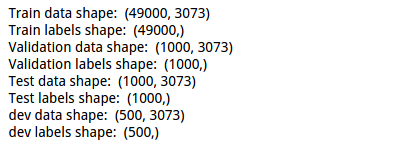
cell 2 读取数据,并显示各个数据的尺寸:
 1 def get_CIFAR10_data(num_training=49000, num_validation=1000, num_test=1000, num_dev=500):
 2   """
 3   Load the CIFAR-10 dataset from disk and perform preprocessing to prepare
 4   it for the linear classifier. These are the same steps as we used for the
 5   SVM, but condensed to a single function.
 6   """
 7   # Load the raw CIFAR-10 data
 8   cifar10_dir = 'cs231n/datasets/cifar-10-batches-py'
 9   X_train, y_train, X_test, y_test = load_CIFAR10(cifar10_dir)
10
11   # subsample the data
12   mask = range(num_training, num_training + num_validation)
13   X_val = X_train[mask]
14   y_val = y_train[mask]
15   mask = range(num_training)
16   X_train = X_train[mask]
17   y_train = y_train[mask]
18   mask = range(num_test)
19   X_test = X_test[mask]
20   y_test = y_test[mask]
21   mask = np.random.choice(num_training, num_dev, replace=False)
22   X_dev = X_train[mask]
23   y_dev = y_train[mask]
24
25   # Preprocessing: reshape the image data into rows
26   X_train = np.reshape(X_train, (X_train.shape[0], -1))
27   X_val = np.reshape(X_val, (X_val.shape[0], -1))
28   X_test = np.reshape(X_test, (X_test.shape[0], -1))
29   X_dev = np.reshape(X_dev, (X_dev.shape[0], -1))
30
31   # Normalize the data: subtract the mean image
32   mean_image = np.mean(X_train, axis = 0)
33   X_train -= mean_image
34   X_val -= mean_image
35   X_test -= mean_image
36   X_dev -= mean_image
37
38   # add bias dimension and transform into columns
39   X_train = np.hstack([X_train, np.ones((X_train.shape[0], 1))])
40   X_val = np.hstack([X_val, np.ones((X_val.shape[0], 1))])
41   X_test = np.hstack([X_test, np.ones((X_test.shape[0], 1))])
42   X_dev = np.hstack([X_dev, np.ones((X_dev.shape[0], 1))])
43
44   return X_train, y_train, X_val, y_val, X_test, y_test, X_dev, y_dev
45
46
47 # Invoke the above function to get our data.
48 X_train, y_train, X_val, y_val, X_test, y_test, X_dev, y_dev = get_CIFAR10_data()
49 print 'Train data shape: ', X_train.shape
50 print 'Train labels shape: ', y_train.shape
51 print 'Validation data shape: ', X_val.shape
52 print 'Validation labels shape: ', y_val.shape
53 print 'Test data shape: ', X_test.shape
54 print 'Test labels shape: ', y_test.shape
55 print 'dev data shape: ', X_dev.shape
56 print 'dev labels shape: ', y_dev.shape
数据维度结果:
cell 3 用for循环实现Softmax的loss function 与grad:
 1 # First implement the naive softmax loss function with nested loops.
 2 # Open the file cs231n/classifiers/softmax.py and implement the
 3 # softmax_loss_naive function.
 4
 5 from cs231n.classifiers.softmax import softmax_loss_naive
 6 import time
 7
 8 # Generate a random softmax weight matrix and use it to compute the loss.
 9 W = np.random.randn(3073, 10) * 0.0001
10 loss, grad = softmax_loss_naive(W, X_dev, y_dev, 0.0)
11
12 # As a rough sanity check, our loss should be something close to -log(0.1).
13 print 'loss: %f' % loss
14 print 'sanity check: %f' % (-np.log(0.1))
对应的py文件的代码:
 1 def softmax_loss_naive(W, X, y, reg):
 2   """
 3   Softmax loss function, naive implementation (with loops)
 4
 5   Inputs have dimension D, there are C classes, and we operate on minibatches
 6   of N examples.
 7
 8   Inputs:
 9   - W: A numpy array of shape (D, C) containing weights.
10   - X: A numpy array of shape (N, D) containing a minibatch of data.
11   - y: A numpy array of shape (N,) containing training labels; y[i] = c means
12     that X[i] has label c, where 0 <= c < C.
13   - reg: (float) regularization strength
14
15   Returns a tuple of:
16   - loss as single float
17   - gradient with respect to weights W; an array of same shape as W
18   """
19   # Initialize the loss and gradient to zero.
20   loss = 0.0
21   dW = np.zeros_like(W)
22
23   #############################################################################
24   # TODO: Compute the softmax loss and its gradient using explicit loops.     #
25   # Store the loss in loss and the gradient in dW. If you are not careful     #
26   # here, it is easy to run into numeric instability. Don't forget the        #
27   # regularization!                                                           #
28   #############################################################################
29   num_calss = W.shape[1]
30   num_train = X.shape[0]
31   buf_e = np.zeros(num_calss)
32 #print buf_e.shape
33
34   for i in xrange(num_train) :
35     for j in xrange(num_calss) :
36   #1*3073 * 3073*1 = 1 >>>10
37       buf_e[j] = np.dot(X[i,:],W[:,j])
38     buf_e -= np.max(buf_e)
39     buf_e = np.exp(buf_e)
40     buf_sum = np.sum(buf_e)
41     buf = buf_e/ buf_sum
42     loss -= np.log(buf[y[i]] )
43     for j in xrange(num_calss):
44         dW[:,j] +=( buf[j] - (j ==y[i]) )*X[i,:].T
45   #regularization with elementwise production
46   loss /= num_train
47   dW /= num_train
48
49   loss += 0.5 * reg * np.sum(W * W)
50   dW +=reg*W
51    #gradient
52
53   #############################################################################
54   #                          END OF YOUR CODE                                 #
55   #############################################################################
56
57   return loss, dW
计算得到的结果:
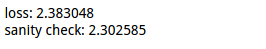
使用了课程上所讲的验证方式。
问题:

cell 4 使用数值计算法对解析法得到的grad进行检验:
 1 # Complete the implementation of softmax_loss_naive and implement a (naive)
 2 # version of the gradient that uses nested loops.
 3 loss, grad = softmax_loss_naive(W, X_dev, y_dev, 0.0)
 4
 5 # As we did for the SVM, use numeric gradient checking as a debugging tool.
 6 # The numeric gradient should be close to the analytic gradient.
 7 from cs231n.gradient_check import grad_check_sparse
 8 f = lambda w: softmax_loss_naive(w, X_dev, y_dev, 0.0)[0]
 9 grad_numerical = grad_check_sparse(f, W, grad, 10)
10
11 # similar to SVM case, do another gradient check with regularization
12 loss, grad = softmax_loss_naive(W, X_dev, y_dev, 1e2)
13 f = lambda w: softmax_loss_naive(w, X_dev, y_dev, 1e2)[0]
14 grad_numerical = grad_check_sparse(f, W, grad, 10)
计算结果:

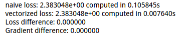
cell 5 使用向量法来实现loss funvtion与grad,并与使用for循环法比较:
 1 # Now that we have a naive implementation of the softmax loss function and its gradient,
 2 # implement a vectorized version in softmax_loss_vectorized.
 3 # The two versions should compute the same results, but the vectorized version should be
 4 # much faster.
 5 tic = time.time()
 6 loss_naive, grad_naive = softmax_loss_naive(W, X_dev, y_dev, 0.00001)
 7 toc = time.time()
 8 print 'naive loss: %e computed in %fs' % (loss_naive, toc - tic)
 9
10 from cs231n.classifiers.softmax import softmax_loss_vectorized
11 tic = time.time()
12 loss_vectorized, grad_vectorized = softmax_loss_vectorized(W, X_dev, y_dev, 0.00001)
13 toc = time.time()
14 print 'vectorized loss: %e computed in %fs' % (loss_vectorized, toc - tic)
15
16 # As we did for the SVM, we use the Frobenius norm to compare the two versions
17 # of the gradient.
18 grad_difference = np.linalg.norm(grad_naive - grad_vectorized, ord='fro')
19 print 'Loss difference: %f' % np.abs(loss_naive - loss_vectorized)
20 print 'Gradient difference: %f' % grad_difference
比较的结果:
向量法的具体代码实现:
 1 def softmax_loss_vectorized(W, X, y, reg):
 2   """
 3   Softmax loss function, vectorized version.
 4
 5   Inputs and outputs are the same as softmax_loss_naive.
 6   """
 7   # Initialize the loss and gradient to zero.
 8   loss = 0.0
 9   dW = np.zeros_like(W)
10   num_calss = W.shape[1]
11   num_train = X.shape[0]
12   #############################################################################
13   # TODO: Compute the softmax loss and its gradient using no explicit loops.  #
14   # Store the loss in loss and the gradient in dW. If you are not careful     #
15   # here, it is easy to run into numeric instability. Don't forget the        #
16   # regularization!                                                           #
17   #############################################################################
18   #500*3073 3073*10 >>>500*10
19   buf_e  = np.dot(X,W)
20   # 10 * 500 - 1*500   T
21   buf_e = np.subtract( buf_e.T , np.max(buf_e , axis = 1) ).T
22   buf_e = np.exp(buf_e)
23   #10*500 - 1*500 T
24   buf_e = np.divide( buf_e.T , np.sum(buf_e , axis = 1) ).T
25   #get loss
26   #print buf.shape
27   loss = - np.sum(np.log ( buf_e[np.arange(num_train),y] ) )
28   #get grad
29   buf_e[np.arange(num_train),y]  -= 1
30   # 3073 * 500 * 500*10
31   loss /=num_train  + 0.5 * reg * np.sum(W * W)
32   dW = np.dot(X.T,buf_e)/num_train + reg*W
33
34   #############################################################################
35   #                          END OF YOUR CODE                                 #
36   #############################################################################
37
38   return loss, dW
cell 6 使用验证集与训练集做超参数选取:
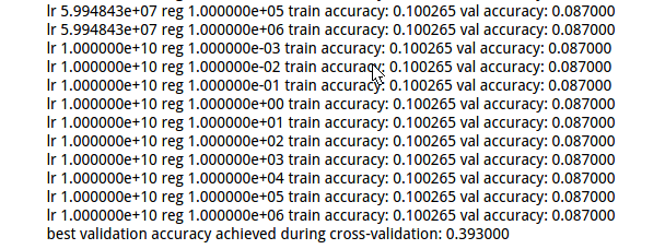
 1 # Use the validation set to tune hyperparameters (regularization strength and
 2 # learning rate). You should experiment with different ranges for the learning
 3 # rates and regularization strengths; if you are careful you should be able to
 4 # get a classification accuracy of over 0.35 on the validation set.
 5 from cs231n.classifiers import Softmax
 6 results = {}
 7 best_val = -1
 8 best_softmax = None
 9 learning_rates = np.logspace(-10, 10, 10)# [1e-7, 2e-7,3e-7,4e-7,5e-7]
10 regularization_strengths = np.logspace(-3, 6, 10) #[1e4,5e4,1e5,5e5,1e6,5e6,1e7,5e7,1e8]
11
12 ################################################################################
13 # TODO:                                                                        #
14 # Use the validation set to set the learning rate and regularization strength. #
15 # This should be identical to the validation that you did for the SVM; save    #
16 # the best trained softmax classifer in best_softmax.                          #
17 ################################################################################
18 iters = 1500
19 for lr in learning_rates:
20     for rs in regularization_strengths:
21         softmax = Softmax()
22         softmax.train(X_train, y_train, learning_rate=lr, reg=rs, num_iters=iters)
23         y_train_pred = softmax.predict(X_train)
24         accu_train = np.mean(y_train == y_train_pred)
25         y_val_pred = softmax.predict(X_val)
26         accu_val = np.mean(y_val == y_val_pred)
27
28         results[(lr, rs)] = (accu_train, accu_val)
29
30         if best_val < accu_val:
31             best_val = accu_val
32             best_softmax = softmax
33 ################################################################################
34 #                              END OF YOUR CODE                                #
35 ################################################################################
36
37 # Print out results.
38 for lr, reg in sorted(results):
39     train_accuracy, val_accuracy = results[(lr, reg)]
40     print 'lr %e reg %e train accuracy: %f val accuracy: %f' % (
41                 lr, reg, train_accuracy, val_accuracy)
42
43 print 'best validation accuracy achieved during cross-validation: %f' % best_val
得到较好的结果:
cell 7 选取较好的超参数的模型,对测试集进行测试,计算准确率:
1 # evaluate on test set
2 # Evaluate the best softmax on test set
3 y_test_pred = best_softmax.predict(X_test)
4 test_accuracy = np.mean(y_test == y_test_pred)
5 print 'softmax on raw pixels final test set accuracy: %f' % (test_accuracy, )
结果:0.378
cell 8 可视化w值:
 1 # Visualize the learned weights for each class
 2 w = best_softmax.W[:-1,:] # strip out the bias
 3 w = w.reshape(32, 32, 3, 10)
 4
 5 w_min, w_max = np.min(w), np.max(w)
 6
 7 classes = ['plane', 'car', 'bird', 'cat', 'deer', 'dog', 'frog', 'horse', 'ship', 'truck']
 8 for i in xrange(10):
 9   plt.subplot(2, 5, i + 1)
10
11   # Rescale the weights to be between 0 and 255
12   wimg = 255.0 * (w[:, :, :, i].squeeze() - w_min) / (w_max - w_min)
13   plt.imshow(wimg.astype('uint8'))
14   plt.axis('off')
15   plt.title(classes[i])
结果:

注:在softmax 与svm的超参数选择时,使用了共同的类,以及类中不同的相应的方法。具体的文件内容与注释如下。
附:通关CS231n企鹅群:578975100 validation:DL-CS231n

