MTCNN算法与代码理解—人脸检测和人脸对齐联合学习

博客：blog.shinelee.me | 博客园 | CSDN

目录

• 写在前面
• 算法Pipeline详解
• 如何训练
  • 损失函数
  • 训练数据准备
  • 多任务学习与在线困难样本挖掘
• 预测过程
• 参考

写在前面

主页：https://kpzhang93.github.io/MTCNN_face_detection_alignment/index.html
论文：https://arxiv.org/abs/1604.02878
代码：官方matlab版、C++ caffe版
第三方训练代码：tensorflow、mxnet

MTCNN，恰如论文标题《Joint Face Detection and Alignment using Multi-task Cascaded Convolutional Networks》所言，采用级联CNN结构，通过多任务学习，同时完成了两个任务——人脸检测和人脸对齐，输出人脸的Bounding Box以及人脸的关键点（眼睛、鼻子、嘴）位置。

MTCNN 又好又快，提出时在FDDB、WIDER FACE和AFLW数据集上取得了当时（2016年4月）最好的结果，速度又快，现在仍被广泛使用作为人脸识别的前端，如InsightFace和facenet。

MTCNN效果为什么好，文中提了3个主要的原因：

1. 精心设计的级联CNN架构（carefully designed cascaded CNNs architecture）
2. 在线困难样本挖掘（online hard sample mining strategy）
3. 人脸对齐联合学习（joint face alignment learning）

下面详细介绍。

算法Pipeline详解

总体而言，MTCNN方法可以概括为：图像金字塔+3阶段级联CNN，如下图所示

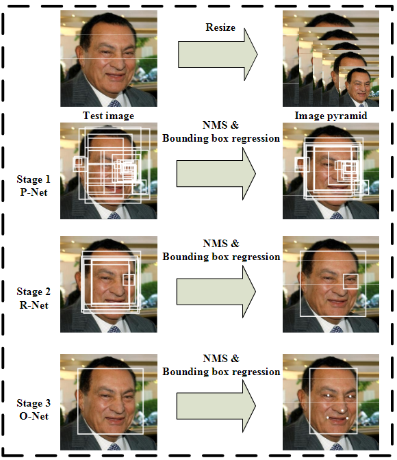
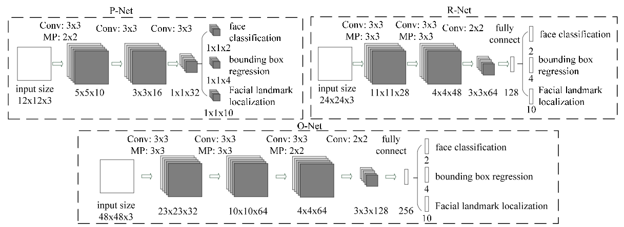
对输入图像建立金字塔是为了检测不同尺度的人脸，通过级联CNN完成对人脸 由粗到细（coarse-to-fine） 的检测，所谓级联指的是 前者的输出是后者的输入，前者往往先使用少量信息做个大致的判断，快速将不是人脸的区域剔除，剩下可能包含人脸的区域交给后面更复杂的网络，利用更多信息进一步筛选，这种由粗到细的方式在保证召回率的情况下可以大大提高筛选效率。下面为MTCNN中级联的3个网络（P-Net、R-Net、O-Net），可以看到它们的网络层数逐渐加深，输入图像的尺寸（感受野）在逐渐变大12→24→48，最终输出的特征维数也在增加32→128→256，意味着利用的信息越来越多。

工作流程是怎样的？
首先，对原图通过双线性插值构建图像金字塔，可以参看前面的博文《人脸检测中，如何构建输入图像金字塔》。构建好金字塔后，将金字塔中的图像逐个输入给P-Net。

• P-Net：其实是个全卷积神经网络（FCN），前向传播得到的特征图在每个位置是个32维的特征向量，用于判断每个位置处约\(12\times12\)大小的区域内是否包含人脸，如果包含人脸，则回归出人脸的Bounding Box，进一步获得Bounding Box对应到原图中的区域，通过NMS保留分数最高的Bounding box以及移除重叠区域过大的Bounding Box。
• R-Net：是单纯的卷积神经网络（CNN），先将P-Net认为可能包含人脸的Bounding Box 双线性插值到\(24\times24\)，输入给R-Net，判断是否包含人脸，如果包含人脸，也回归出Bounding Box，同样经过NMS过滤。
• O-Net：也是纯粹的卷积神经网络（CNN），将R-Net认为可能包含人脸的Bounding Box 双线性插值到\(48\times 48\)，输入给O-Net，进行人脸检测和关键点提取。

需要注意的是：

1. face classification判断是不是人脸使用的是softmax，因此输出是2维的，一个代表是人脸，一个代表不是人脸
2. bounding box regression回归出的是bounding box左上角和右下角的偏移\(dx1, dy1, dx2, dy2\)，因此是4维的
3. facial landmark localization回归出的是左眼、右眼、鼻子、左嘴角、右嘴角共5个点的位置，因此是10维的
4. 在训练阶段，3个网络都会将关键点位置作为监督信号来引导网络的学习， 但在预测阶段，P-Net和R-Net仅做人脸检测，不输出关键点位置（因为这时人脸检测都是不准的），关键点位置仅在O-Net中输出。
5. Bounding box和关键点输出均为归一化后的相对坐标，Bounding Box是相对待检测区域（R-Net和O-Net是相对输入图像），归一化是相对坐标除以检测区域的宽高，关键点坐标是相对Bounding box的坐标，归一化是相对坐标除以Bounding box的宽高，这里先建立起初步的印象，具体可以参看后面准备训练数据部分和预测部分的代码细节。

MTCNN效果好的第1个原因是精心设计的级联CNN架构，其实，级联的思想早已有之，而使用级联CNN进行人脸检测的方法是在2015 CVPR《A convolutional neural network cascade for face detection》中被率先提出，MTCNN与之的差异在于：

• 减少卷积核数量（层内）
• 将\(5\times 5\)的卷积核替换为\(3\times 3\)
• 增加网络深度

这样使网络的表达能力更强，同时运行时间更少。

MTCNN效果好的后面2个原因在线困难样本挖掘和人脸对齐联合学习将在下一节介绍。

如何训练

损失函数

MTCNN的多任务学习有3个任务，1个分类2个回归，分别为face classification、bounding box regression以及facial landmark localization，分类的损失函数使用交叉熵损失，回归的损失函数使用欧氏距离损失，如下：

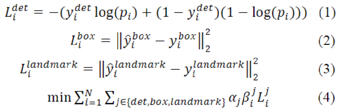
对于第\(i\)个样本，\(L_i^{det}\)为判断是不是人脸的交叉熵损失，\(L_i^{box}\)为bounding box回归的欧式距离损失，\(L_i^{landmark}\)为关键点定位的欧氏距离损失，任务间权重通过\(\alpha_j\)协调，配置如下：

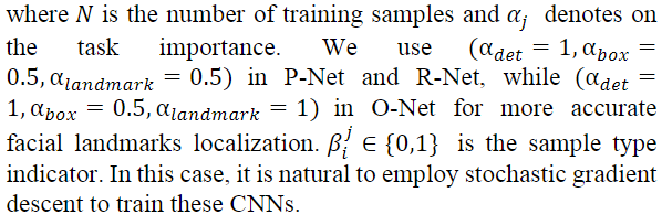
同时，训练数据中有含人脸的、有不含人脸的、有标注了关键点的、有没标注关键点的，不同数据能参与的训练任务不同，比如不含人脸的负样本自然无法用于训练bounding box回归和关键点定位，于是有了\(\beta_i^j \in \{ 0, 1\}\)，指示每个样本能参与的训练任务，例如对于不含人脸的负样本其\(\beta_i^{det}=1, \beta_i^{box}=0, \beta_i^{landmark}=0\)。

至此，我们已经清楚了MTCNN多任务学习的损失函数。

训练数据准备

MTCNN准备了4种训练数据：

1. Negatives：与ground-truth faces的\(IOU < 0.3\)的图像区域，lable = 0
2. Positives：与ground-truth faces的\(IOU \ge 0.65\)的图像区域，lable = 1
3. Part faces：与ground-truth faces的\(0.4 \le IOU < 0.65\)的图像区域，lable = -1
4. Landmark faces：标记了5个关键点的人脸图像，lable = -2

这4种数据是如何组织的呢？以MTCNN-Tensorflow为例：

Since MTCNN is a Multi-task Network,we should pay attention to the format of training data.The format is:
[path to image] [cls_label] [bbox_label] [landmark_label]
For neg sample, cls_label=0, bbox_label=[0,0,0,0], landmark_label=[0,0,0,0,0,0,0,0,0,0].
For pos sample, cls_label=1, bbox_label(calculate), landmark_label=[0,0,0,0,0,0,0,0,0,0].
For part sample, cls_label=-1, bbox_label(calculate), landmark_label=[0,0,0,0,0,0,0,0,0,0].
For landmark sample, cls_label=-2, bbox_label=[0,0,0,0], landmark_label(calculate).

数量之比依次为\(3:1:1:2\)，其中，Negatives、Positives和Part faces通过WIDER FACE数据集crop得到，landmark faces通过CelebA数据集crop得到，先crop区域，然后看这个区域与哪个ground-truth face的IOU最大，根据最大IOU来生成label，比如小于0.3的标记为negative。

P-Net训练数据的准备可以参见gen_12net_data.py、gen_landmark_aug_12.py、gen_imglist_pnet.py和gen_PNet_tfrecords.py，代码很直观，这里略过crop过程，重点介绍bounding box label和landmark label的生成。下面是gen_12net_data.py和gen_landmark_aug_12.py中的代码片段，bounding box 和 landmark 的label为归一化后的相对坐标，offset_x1, offset_y1, offset_x2, offset_y2为bounding box的label，使用crop区域的size进行归一化，rv为landmark的label，使用bbox的宽高进行归一化，注意两者的归一化是不一样的，具体见代码：

## in gen_12net_data.py
# pos and part face size [minsize*0.8,maxsize*1.25]
size = npr.randint(int(min(w, h) * 0.8), np.ceil(1.25 * max(w, h)))

# delta here is the offset of box center
if w<5:
    print (w)
    continue
#print (box)
delta_x = npr.randint(-w * 0.2, w * 0.2)
delta_y = npr.randint(-h * 0.2, h * 0.2)

#show this way: nx1 = max(x1+w/2-size/2+delta_x)
# x1+ w/2 is the central point, then add offset , then deduct size/2
# deduct size/2 to make sure that the right bottom corner will be out of
nx1 = int(max(x1 + w / 2 + delta_x - size / 2, 0))
#show this way: ny1 = max(y1+h/2-size/2+delta_y)
ny1 = int(max(y1 + h / 2 + delta_y - size / 2, 0))
nx2 = nx1 + size
ny2 = ny1 + size

if nx2 > width or ny2 > height:
    continue 
crop_box = np.array([nx1, ny1, nx2, ny2])
#yu gt de offset
##### x1 y1 x2 y2 为 ground truth bbox， nx1 ny1 nx2 ny2为crop的区域，size为crop的区域size ######
offset_x1 = (x1 - nx1) / float(size) 
offset_y1 = (y1 - ny1) / float(size)
offset_x2 = (x2 - nx2) / float(size)
offset_y2 = (y2 - ny2) / float(size)
#crop
cropped_im = img[ny1 : ny2, nx1 : nx2, :]
#resize
resized_im = cv2.resize(cropped_im, (12, 12), interpolation=cv2.INTER_LINEAR)
##########################################################################

## in gen_landmark_aug_12.py
#normalize land mark by dividing the width and height of the ground truth bounding box
# landmakrGt is a list of tuples
for index, one in enumerate(landmarkGt):
    # (( x - bbox.left)/ width of bounding box, (y - bbox.top)/ height of bounding box
    rv = ((one[0]-gt_box[0])/(gt_box[2]-gt_box[0]), (one[1]-gt_box[1])/(gt_box[3]-gt_box[1]))
    # put the normalized value into the new list landmark
    landmark[index] = rv

需要注意的是，对于P-Net，其为FCN，预测阶段输入图像可以为任意大小，但在训练阶段，使用的训练数据均被resize到\(12\times 12\)，以便于控制正负样本的比例（避免数据不平衡）。

因为是级联结构，训练要分阶段依次进行，训练好P-Net后，用P-Net产生的候选区域来训练R-Net，训练好R-Net后，再生成训练数据来训练O-Net。P-Net训练好之后，根据其结果准备R-Net的训练数据，R-Net训练好之后，再准备O-Net的训练数据，过程是类似的，具体可以参见相关代码，这里就不赘述了。

多任务学习与在线困难样本挖掘

4种训练数据参与的训练任务如下：

• Negatives和Positives用于训练face classification
• Positives和Part faces用于训练bounding box regression
• landmark faces用于训练facial landmark localization

据此来设置\(\beta_i^j\)，对每一个样本看其属于那种训练数据，对其能参与的任务将\(\beta\)置为1，不参与的置为0。

至于在线困难样本挖掘，仅在训练face/non-face classification时使用，具体做法是：对每个mini-batch的数据先通过前向传播，挑选损失最大的前70%作为困难样本，在反向传播时仅使用这70%困难样本产生的损失。文中的实验表明，这样做在FDDB数据级上可以带来1.5个点的性能提升。

具体怎么实现的？这里以MTCNN-Tensorflow / train_models / mtcnn_model.py代码为例，用label来指示是哪种数据，下面为代码，重点关注valid_inds和loss（square_error）的计算（对应\(\beta_i^j\)），以及cls_ohem中的困难样本挖掘。

# in mtcnn_model.py]
# pos=1, neg=0, part=-1, landmark=-2
# 通过cls_ohem, bbox_ohem, landmark_ohem来计算损失
num_keep_radio = 0.7 # mini-batch前70%做为困难样本

# face/non-face 损失，注意在线困难样本挖掘（前70%）
def cls_ohem(cls_prob, label):
    zeros = tf.zeros_like(label)
    #label=-1 --> label=0net_factory

    #pos -> 1, neg -> 0, others -> 0
    label_filter_invalid = tf.where(tf.less(label,0), zeros, label)
    num_cls_prob = tf.size(cls_prob)
    cls_prob_reshape = tf.reshape(cls_prob,[num_cls_prob,-1])
    label_int = tf.cast(label_filter_invalid,tf.int32)
    # get the number of rows of class_prob
    num_row = tf.to_int32(cls_prob.get_shape()[0])
    #row = [0,2,4.....]
    row = tf.range(num_row)*2
    indices_ = row + label_int
    label_prob = tf.squeeze(tf.gather(cls_prob_reshape, indices_))
    loss = -tf.log(label_prob+1e-10)
    zeros = tf.zeros_like(label_prob, dtype=tf.float32)
    ones = tf.ones_like(label_prob,dtype=tf.float32)
    # set pos and neg to be 1, rest to be 0
    valid_inds = tf.where(label < zeros,zeros,ones)
    # get the number of POS and NEG examples
    num_valid = tf.reduce_sum(valid_inds)

    ###### 困难样本数量 #####
    keep_num = tf.cast(num_valid*num_keep_radio,dtype=tf.int32)
    #FILTER OUT PART AND LANDMARK DATA
    loss = loss * valid_inds
    loss,_ = tf.nn.top_k(loss, k=keep_num) ##### 仅取困难样本反向传播 #####
    return tf.reduce_mean(loss)

# bounding box损失
#label=1 or label=-1 then do regression
def bbox_ohem(bbox_pred,bbox_target,label):
    '''

    :param bbox_pred:
    :param bbox_target:
    :param label: class label
    :return: mean euclidean loss for all the pos and part examples
    '''
    zeros_index = tf.zeros_like(label, dtype=tf.float32)
    ones_index = tf.ones_like(label,dtype=tf.float32)
    # keep pos and part examples
    valid_inds = tf.where(tf.equal(tf.abs(label), 1),ones_index,zeros_index)
    #(batch,)
    #calculate square sum
    square_error = tf.square(bbox_pred-bbox_target)
    square_error = tf.reduce_sum(square_error,axis=1)
    #keep_num scalar
    num_valid = tf.reduce_sum(valid_inds)
    #keep_num = tf.cast(num_valid*num_keep_radio,dtype=tf.int32)
    # count the number of pos and part examples
    keep_num = tf.cast(num_valid, dtype=tf.int32)
    #keep valid index square_error
    square_error = square_error*valid_inds
    # keep top k examples, k equals to the number of positive examples
    _, k_index = tf.nn.top_k(square_error, k=keep_num)
    square_error = tf.gather(square_error, k_index)

    return tf.reduce_mean(square_error)

# 关键点损失
def landmark_ohem(landmark_pred,landmark_target,label):
    '''
    :param landmark_pred:
    :param landmark_target:
    :param label:
    :return: mean euclidean loss
    '''
    #keep label =-2  then do landmark detection
    ones = tf.ones_like(label,dtype=tf.float32)
    zeros = tf.zeros_like(label,dtype=tf.float32)
    valid_inds = tf.where(tf.equal(label,-2),ones,zeros) ##### 将label=-2的置为1，其余为0 #####
    square_error = tf.square(landmark_pred-landmark_target)
    square_error = tf.reduce_sum(square_error,axis=1)
    num_valid = tf.reduce_sum(valid_inds)
    #keep_num = tf.cast(num_valid*num_keep_radio,dtype=tf.int32)
    keep_num = tf.cast(num_valid, dtype=tf.int32)
    square_error = square_error*valid_inds # 在计算landmark_ohem损失时只计算beta=1的 #####
    _, k_index = tf.nn.top_k(square_error, k=keep_num)
    square_error = tf.gather(square_error, k_index)
    return tf.reduce_mean(square_error)

多任务学习的代码片段如下：

# in train.py
if net == 'PNet':
    image_size = 12
    radio_cls_loss = 1.0;radio_bbox_loss = 0.5;radio_landmark_loss = 0.5;
elif net == 'RNet':
    image_size = 24
    radio_cls_loss = 1.0;radio_bbox_loss = 0.5;radio_landmark_loss = 0.5;
else:
    radio_cls_loss = 1.0;radio_bbox_loss = 0.5;radio_landmark_loss = 1;
    image_size = 48

# ...
# 多任务联合损失
total_loss_op  = radio_cls_loss*cls_loss_op + radio_bbox_loss*bbox_loss_op + radio_landmark_loss*landmark_loss_op + L2_loss_op
train_op, lr_op = train_model(base_lr, total_loss_op, num)

def train_model(base_lr, loss, data_num):
    """
    train model
    :param base_lr: base learning rate
    :param loss: loss
    :param data_num:
    :return:
    train_op, lr_op
    """
    lr_factor = 0.1
    global_step = tf.Variable(0, trainable=False)
    #LR_EPOCH [8,14]
    #boundaried [num_batch,num_batch]
    boundaries = [int(epoch * data_num / config.BATCH_SIZE) for epoch in config.LR_EPOCH]
    #lr_values[0.01,0.001,0.0001,0.00001]
    lr_values = [base_lr * (lr_factor ** x) for x in range(0, len(config.LR_EPOCH) + 1)]
    #control learning rate
    lr_op = tf.train.piecewise_constant(global_step, boundaries, lr_values)
    optimizer = tf.train.MomentumOptimizer(lr_op, 0.9)
    train_op = optimizer.minimize(loss, global_step)
    return train_op, lr_op

以上对应论文中的损失函数。

预测过程

预测过程与算法Pipeline详解一节讲述的一致，直接看一下官方matlab代码，这里重点关注P-Net FCN是如何获得Bounding box的，以及O-Net最终是如何得到landmark的，其余部分省略。

将图像金字塔中的每张图像输入给P-Net，若当前输入图像尺寸为\(M\times N\)，在bounding box regression分支上将得到一个3维张量\(m\times n \times 4\)，共有\(m\times n\)个位置，每个位置对应输入图像中一个\(12\times 12\)的区域，而输入图像相对原图的尺度为scale，进一步可以获得每个位置对应到原图中的区域范围，如下所示：

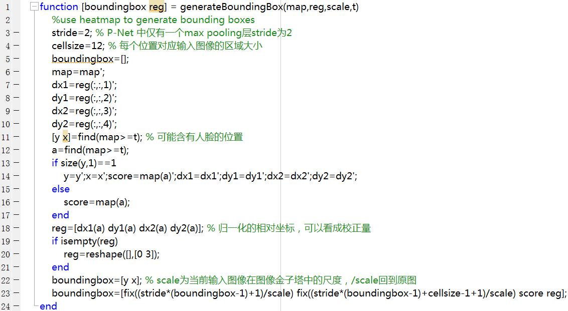
而每个位置处都有个\(4\)维的向量，其为bounding box左上角和右下角的偏移dx1, dy1, dx2, dy2，通过上面的训练过程，我们知道它们是归一化之后的相对坐标，通过对应的区域以及归一化后的相对坐标就可以获得原图上的bounding box，如下所示，dx1, dy1, dx2, dy2为归一化的相对坐标，求到原图中的bounding box坐标的过程为生成训练数据bounding box label的逆过程。

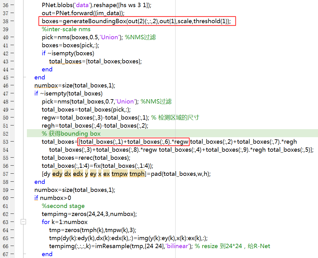
landmark位置通过O-Net输出得到，将人脸候选框resize到\(48\times 48\)输入给O-Net，先获得bounding box（同上），因为O-Net输出的landmark也是归一化后的相对坐标，通过bounding box的长宽和bounding box左上角求取landmark 在原图中的位置，如下所示：

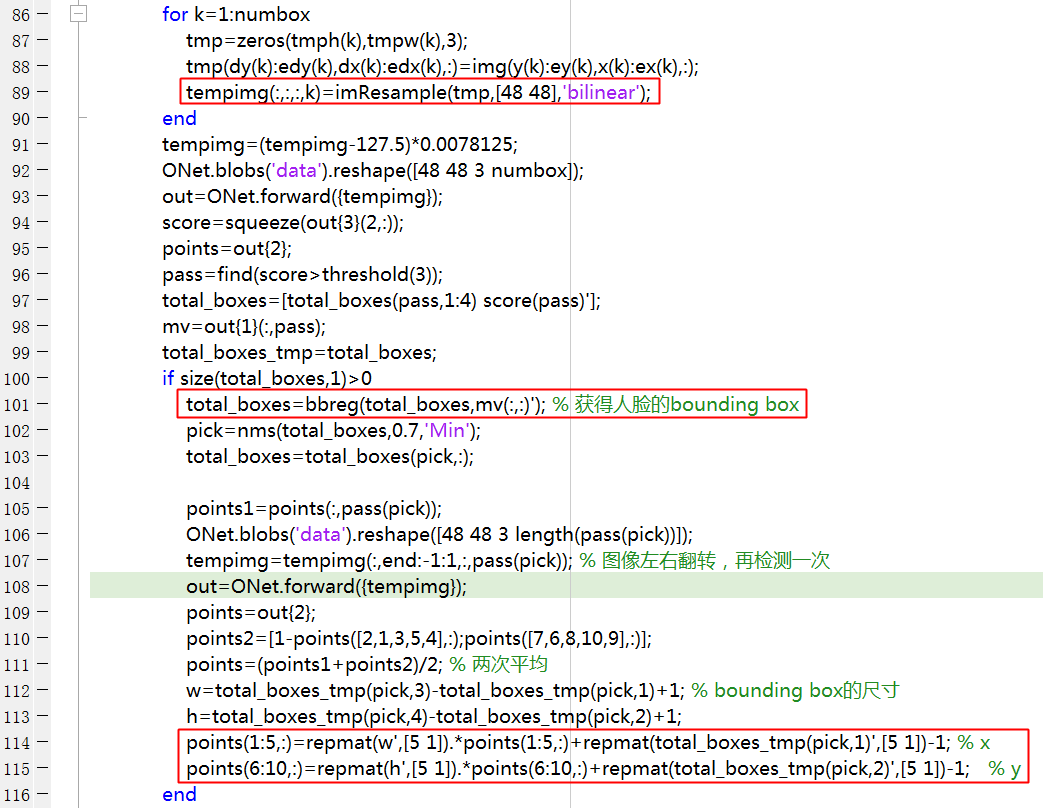
至此，预测过程中的要点也介绍完毕了，以上。

参考

• Joint Face Detection and Alignment using Multi-task Cascaded Convolutional Networks
• 官方matlab code
• 第三方tensorflow code