Adaptive Thresholding & Otsu’s Binarization
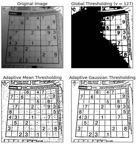
Adaptive Thresholding
Adaptive Method - It decides how thresholding value is calculated.
- cv2.ADAPTIVE_THRESH_MEAN_C : threshold value is the mean of neighbourhood area.
- cv2.ADAPTIVE_THRESH_GAUSSIAN_C : threshold value is the weighted sum of neighbourhood values where weights are a gaussian window.
Otsu’s Binarization
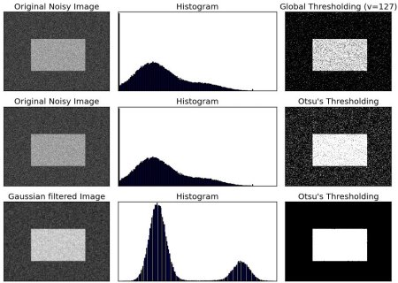
In global thresholding, we used an arbitrary value for threshold value, right? So, how can we know a value we selected is good or not? Answer is, trial and error method. But consider a bimodal image (In simple words, bimodal image is an image whose histogram has two peaks). For that image, we can approximately take a value in the middle of those peaks as threshold value, right ? That is what Otsu binarization does. So in simple words, it automatically calculates a threshold value from image histogram for a bimodal image. (For images which are not bimodal, binarization won’t be accurate.)
Check out below example. Input image is a noisy image. In first case, I applied global thresholding for a value of 127. In second case, I applied Otsu’s thresholding directly. In third case, I filtered image with a 5x5 gaussian kernel to remove the noise, then applied Otsu thresholding. See how noise filtering improves the result.
How Otsu's Binarization Works?
This section demonstrates a Python implementation of Otsu's binarization to show how it works actually. If you are not interested, you can skip this.
Since we are working with bimodal images, Otsu's algorithm tries to find a threshold value (t) which minimizes the weighted within-class variance given by the relation :
\[\sigma_w^2(t) = q_1(t)\sigma_1^2(t)+q_2(t)\sigma_2^2(t)\]
where
\[q_1(t) = \sum_{i=1}^{t} P(i) \quad \& \quad q_1(t) = \sum_{i=t+1}^{I} P(i)\]
\[\mu_1(t) = \sum_{i=1}^{t} \frac{iP(i)}{q_1(t)} \quad \& \quad \mu_2(t) = \sum_{i=t+1}^{I} \frac{iP(i)}{q_2(t)}\]
\[\sigma_1^2(t) = \sum_{i=1}^{t} [i-\mu_1(t)]^2 \frac{P(i)}{q_1(t)} \quad \& \quad \sigma_2^2(t) = \sum_{i=t+1}^{I} [i-\mu_1(t)]^2 \frac{P(i)}{q_2(t)}\]
It actually finds a value of t which lies in between two peaks such that variances to both classes are minimum. It can be simply implemented in Python as follows:
   img = cv2.imread('noisy2.png',0)
   blur = cv2.GaussianBlur(img,(5,5),0)

   # find normalized_histogram, and its cumulative distribution function
   hist = cv2.calcHist([blur],[0],None,[256],[0,256])
   hist_norm = hist.ravel()/hist.max()
   Q = hist_norm.cumsum()

   bins = np.arange(256)

   fn_min = np.inf
   thresh = -1

   for i in xrange(1,256):
      p1,p2 = np.hsplit(hist_norm,[i]) # probabilities
      q1,q2 = Q[i],Q[255]-Q[i] # cum sum of classes
      b1,b2 = np.hsplit(bins,[i]) # weights

      # finding means and variances
      m1,m2 = np.sum(p1*b1)/q1, np.sum(p2*b2)/q2
      v1,v2 = np.sum(((b1-m1)**2)*p1)/q1,np.sum(((b2-m2)**2)*p2)/q2

      # calculates the minimization function
      fn = v1*q1 + v2*q2
      if fn < fn_min:
         fn_min = fn
         thresh = i

   # find otsu's threshold value with OpenCV function
   ret, otsu = cv2.threshold(blur,0,255,cv2.THRESH_BINARY+cv2.THRESH_OTSU)
   print thresh,ret