Robust Locally Weighted Regression 鲁棒局部加权回归 -R实现

鲁棒局部加权回归

【转载时请注明来源】：http://www.cnblogs.com/runner-ljt/

    Ljt

    作为一个初学者，水平有限，欢迎交流指正。

 

 算法参考文献：

 （1） Robust Locally Weighted Regression and Smoothing Scatterplots (Willism_S.Cleveland)

 （2） 数据挖掘中强局部加权回归算法实现 (虞乐,肖基毅)

 

 

 

R实现

#Robust Locally Weighted Regression 鲁棒局部加权回归

# 一元样本值x,y ;待预测样本点xp ;f局部加权窗口大小（一般取1/3~2/3）;d局部加权回归阶数;
#time鲁棒局部加权回归次数(一般取2就几乎可以满足收敛);
#step梯度下降法固定步长;error梯度下降法终止误差;maxiter最大迭代次数
RobustLWRegression<-function(x,y,xp,f,d,time,step,error,maxiter){
  
  m<-nrow(x)
  r<-floor(f*m) #窗口内的样本量
  xl<-abs(x-xp)
  xll<-xl[order(xl)]
  hr<-xll[r]  #h为离xp第r个最近的样本到xp的距离
  
  #三次权值函数(几乎在所有情况下都能够提供充分平滑)
  xk<-(x-xp)/hr
  w<-ifelse(abs(xk)<1,(1-abs(xk^3))^3,0)
  
  #d次回归函数
  for(i in 2:d){
    x<-cbind(x,x^i)
  }
  x<-cbind(1,x)
  n<-ncol(x)
  
  #梯度下降法（固定步长）求局部加权回归的系数
  theta<-matrix(0,n,1) #theta 初始值都设置为0
  iter<-0
  newerror<-1   
  while((newerror>error)|(iter<maxiter)){
    iter<-iter+1
    h<-x%*%theta   
    des<-t(t(w*(h-y))%*%x)      #局部加权梯度     
    new_theta<-theta-step*des   #直接设置固定步长   
    newerror<-t(theta-new_theta)%*%(theta-new_theta)
    theta<-new_theta      
  }
  
  #time次鲁棒局部加权回归
  for(i in 1:time){
    e<-y-x%*%theta   
    s<-median(e) 
    #四次权值函数
    xb<-e/(6*s)
    R_w<-ifelse(abs(xb)<1,(1-xb^2)^2,0)
    
    #梯度下降法求鲁棒加权局部回归
    R_theta<-matrix(0,n,1) #theta 初始值都设置为0
    R_iter<-0
    R_newerror<-1
    while((R_newerror>error)|(R_iter<maxiter)){
      R_iter<-R_iter+1
      R_h<-x%*%R_theta   
      R_des<-t(t(w*R_w*(R_h-y))%*%x)    #鲁棒局部加权梯度     
      R_new_theta<-R_theta-step*R_des   #直接设置固定步长   
      R_newerror<-t(R_theta-R_new_theta)%*%(R_theta-R_new_theta)
      R_theta<-R_new_theta      
    }
    theta<-R_theta   
  }
  
  
  for(i in 2:d){
     xp<-cbind(xp,xp^i)
  }
  xp<-cbind(1,xp)
  yp<-xp%*%theta
  # costfunction<-t(x%*%theta-y)%*%(x%*%theta-y)
  # result<-list(yp,theta,iter,costfunction)
  # names(result)<-c('拟合值','系数','迭代次数','误差')
  # result
  yp
  
}

　　

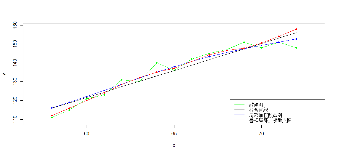
实例比较 线性回归、局部加权线性回归和鲁棒局部加权线性回归：

>
> t(x)
     [,1] [,2] [,3] [,4] [,5] [,6] [,7] [,8] [,9] [,10] [,11] [,12] [,13] [,14] [,15]
[1,]   58   59   60   61   62   63   64   65   66    67    68    69    70    71    72
> t(y)
     [,1] [,2] [,3] [,4] [,5] [,6] [,7] [,8] [,9] [,10] [,11] [,12] [,13] [,14] [,15]
[1,]  111  115  121  123  131  130  140  136  142   145   147   151   148   151   148
> 
> lm(y~x)

Call:
lm(formula = y ~ x)

Coefficients:
(Intercept)            x  
    -50.245        2.864  

> yy<--50.245+2.864*x
> 
> plot(x,y,col='green',pch=20,xlim=c(57,73),ylim=c(109,159))
> lines(x,y,col='green')
> lines(x,yy,col='black')
> 
> g<-apply(x,1,function(xp){LWLRegression(x,y,xp,3,1e-7,100000,stepmethod=F,step=0.00001,alpha=0.25,beta=0.8)})
>
> points(x,g,col='blue',pch=20)
> lines(x,g,col='blue')
>
> gg<-apply(x,1,function(xp){RobustLWRegression(x,y,xp,0.6,2,2,0.00000001,1e-7,10000)})
>
> points(x,gg,col='red',pch=20)
> lines(x,gg,col='red')

> legend('bottomright',legend=c('散点图','拟合直线','局部加权散点图','鲁棒局部加权散点图'),lwd=1,col=c('green','black','blue','red'))
>