
逻辑回归之信用卡
背景:有人利用信用卡欺诈,数据给出了28W多个样本,每一个样本有20多个因素数据和最终是否欺诈的结论。
 1 import numpy as np
 2 import pandas as pd
 3 import matplotlib.pyplot as plt
 4 #导入相关库文件
 5
 6 data = pd.read_csv('creditcard.csv')  #读取文件
 7 print(data.shape)  #打印下文件内容是几行几列
 8 count_class = pd.value_counts(data['Class'],sort = True).sort_index()
 9 #pd.value_counts()对数据集中的['Class']列进行数学统计,统计其中每一类数据出现的个数。
10 #sort_index()是根据索引进行排序,在这个数据集中好像没有什么意义
11 print (count_class)
 1 from sklearn.preprocessing import StandardScaler
 2 # 导入sklearn数据预处理模块,sklearn是机器学期很重的一个库,有时间还是需要着重学习一下
 3 data['normAmount'] = StandardScaler().fit_transform(data['Amount'].values.reshape(-1,1))   # -1表示系统自动计算得到的行,1表示1列
 4 #StandardScaler().fit_transform是sklearn里可将数据标准化的函数,和scale()的功能类似,都可以将数据标准化,具体可以百度
 5 #https://blog.csdn.net/weixin_38278334/article/details/82971752    .fit_transform的应用
 6 #.values是将前边的字典转成数组,也就是转成list。.reshape(-1,1)是将前边的.list转成n行,1列,-1是不指定行数,自动计算得出n
 7 #再将reshape之后的list赋值给data['normAmount'],等于为数据集多增加了一列。
 8 data = data.drop(['Time','Amount'],axis = 1)
 9 #观察数据发现,“Time”这一列没有什么作用,所以删除,“Amount”每个样本之间差距比较大,应将其标准化,
10 #结合上一行,实际就是把['Amount']一列进行标准化,并改名为normAmount。
通过观察数据发现,Class=0的样本有284315个,Class=1的样本有492个,典型的样本不均衡现象。处理方法有两种:过采样和下采样。过采样:增加Class=1的样本数量,增加至和Class=0一样多;下采样:减少Class=0的样本数量,减少至和Class=1的数量相同。
 1 X = data.loc[:,data.columns != 'Class']  #选取非“Class”列,目的是将Class视为标签
 2 #注意.loc和.iloc的区别。iloc主要使用数字来索引数据,不能使用字符型的标签来索引数据。
 3 #loc只能使用字符型标签来索引数据,不能使用数字来索引数据。特殊情况:当dataframe的行标签或列标签为数字时,loc就可以来索引
 4 #如果对数据很熟悉
 5 y = data.loc[:,data.columns == 'Class']    # y 为标签,即类别
 6 number_records_fraud = len(data[data.Class==1])  #统计异常值的个数
 7 #print (number_records_fraud)  # 492 个
 8 fraud_indices = np.array(data[data.Class == 1].index)
 9 #fraud_indices值是取原数据所有Class=1的样本的索引,并转为array的形式。
10 #fraud_indices是所有Class=1的行索引
11 normal_indices = data[data.Class == 0].index   # 记录正常值的索引
12 normal_indices = np.array(normal_indices)
13 #normal_indices是取原数据所有Class=0的样本的索引,并转为array的格式。
14 random_normal_indices =np.random.choice(normal_indices,number_records_fraud,replace = False)
15 #目的是从正常值的索引中,选择和异常值相等个数的样本。
16 #np.random.choice()功能是在第一个参数normal_indices内随机去第二个参数number_records_fraud个数据,number_records_fraud是Class=1的样本数量
17 #random_normal_indices = np.array(random_normal_indices)
18 under_sample_indices = np.concatenate([fraud_indices,random_normal_indices])
19 #np.concatenate是将两个array类型拼接成一个array,类似于append,但是适合大批量数据拼接.注意参数外有一个括号,可以help查询使用方法。
20 under_sample_data = data.iloc[under_sample_indices,:]
21 #under_sample_indices是组合好的新的数据的索引,是一个array,iloc是根据索引找到该数据
22 #under_sample_data最终的值是组合好的数据的新的数据集,是一个数据集
23 X_undersample = under_sample_data.iloc[:, under_sample_data.columns != 'Class']  # 下采样后的训练集
24 #找到新数据集under_sample_data中Class=1的所有列
25 y_undersample = under_sample_data.iloc[:, under_sample_data.columns == 'Class']  # 下采样后的标签
26 #找到新数据集under_sample_data中Class=0的所有列
27 print(len(under_sample_data[under_sample_data.Class == 1]) / len(under_sample_data))  # 正负样本的比例都是 0.5
28 #under_sample_data.Class == 1是个布尔值的array,under_sample_data[]取到under_sample_data中Class=1的所有数据
其实不难发现,上边的代码很多,其实就作了一件事,下采样。随机取Class=0中的若干个样本(数量等于Class=1的数量),重新组合数据。
 1 from sklearn.model_selection import train_test_split
 2 #新版本的要用sklearn.model_selection,网上很多用的是老版本的库,会报错
 3 # from sklearn.cross_validation import train_test_split
 4 # ModuleNotFoundError: No module named 'sklearn.cross_validation'
 5 X_train,X_test,y_train,y_test = train_test_split(X,y,test_size = 0.3,random_state = 0)
 6 #将原始数据按照参数test_size比例切割为训练集和测试集。
 7 X_train_undersample, X_test_undersample, y_train_undersample, y_test_undersample = train_test_split(
 8     X_undersample, y_undersample, test_size=0.3, random_state=0)
 9 #将下采样后的数据按照参数test_size比例切割为训练集和测试集。
10 #这是数据分析预测很重要的一部。将数据分为两部分,第一部分是预测模型用的,第二部分是模型确定后,用来拟合数据,评估模型好坏的。
下一部分代码是比较核心的一部分,用sklearn库里的函数来建立模型。
 1 def printing_Kfold_scores(x_train_data,y_train_data):
 2     fold = KFold(5,shuffle=False)
 3     #KFold就是建立一个交叉验证的模型。没有将数据集代入参数。5的意思是切成5部分,其中4部分和1部分各位1组。
 4     c_param_range = [0.01,0.1,1,10,100]
 5     #惩罚项,在逻辑回归中可以设置惩罚项,分为l1和l2两种。简单来说,l1可以防止过拟合现象(过拟合就是训练接表现很好,但是测试集表现很差)
 6     #l2可以突出某一个参数的权重。惩罚项是需要人为设定的,这里设置多个惩罚项参数,可以对比哪一更好。
 7     results_table = pd.DataFrame(index = range(len(c_param_range),2),columns = ['C_parameter','Mean recall score'])
 8     #建立一个新的DataFrame,行索引是[0,1,2,3,4],列是['C_parameter','Mean recall score'],
 9     #'C_parameter'储存惩罚项参数,'Mean recall score'储存在这一惩罚项参数下的平均recall值
10     #recall值反应预测是否准确。例如10个病人,预测出来了8个,recall=80%
11     #其实index = range(len(c_param_range),2)并没有什么用,因为具体有多少行是由c_param_range内容确定的。
12     results_table['C_parameter'] = c_param_range
13     j = 0
14     for c_param in c_param_range:
15         #此循环的内容是惩罚项参数,也就是计算一种交叉验证情况下的,5种惩罚项参数的recall值
16         print('------------------------------------------')
17         print('C parameter:', c_param)
18         print('-------------------------------------------')
19         print('')
20         recall_accs = []#建立新的array,后后续计算每一种惩罚项参数下的recall做准备
21         for iteration, indices in enumerate(fold.split(x_train_data),start=1):
22             #iteration=[1,2,3,4,5],enumerate有一个参数(start=1),从1开始数
23             lr = LogisticRegression(C=c_param, penalty='l1', solver='liblinear', max_iter=10000)
24             # 使用特定的C参数调用逻辑回归模型
25             # 参数 solver=’liblinear’ 消除警告
26             # 出现警告:模型未能收敛 ,请增加收敛次数
27             #  ConvergenceWarning: Liblinear failed to converge, increase the number of iterations.
28             #  "the number of iterations.", ConvergenceWarning)
29             #  增加参数 max_iter 默认1000
30             lr.fit(x_train_data.iloc[indices[0], :], y_train_data.iloc[indices[0], :].values.ravel())
31             #例如,交叉验证,分为5组数据[0,1,2,3,4],可以分为[0,1,2,3]和[4],[4,1,2,3]和[0],[0,4,2,3]和[1],[0,1,4,3]和[2],[0,1,2,4]和[3]
32             #indices[0]是[[0,1,2,3],[4,1,2,3],[0,4,2,3],[0,1,4,3]],indices[1]是[[4],[0],[1],[2]]
33             #注意,0、1、2、3、4只是索引,KFold分的是索引!
34             # Use the training data to fit the model. In this case, we use the portion
35             # of the fold to train the model with indices[0], We then predict on the
36             # portion assigned as the 'test cross validation' with indices[1]
37
38             y_pred_undersample = lr.predict(x_train_data.iloc[indices[1], :].values)
39             #利用模型预测数据。输入是x_train_data.iloc[indices[1],也就是前边分好的,在交叉验证里每组数据的第二部分。
40             #predict返回的是一个大小为n的一维数组,第i个预测样本的标签;
41             # Predict values using the test indices in the training data
42
43             # Calculate the recall score and append it to a list for recall scores
44             # representing the current c_parameter
45             recall_acc = recall_score(y_train_data.iloc[indices[1], :].values, y_pred_undersample)
46             #计算召回率,y_train_data.iloc[indices[1], :]是真实的数据,y_pred_undersample是预测的数据
47             recall_accs.append(recall_acc)
48             #把刚刚计算完的一种交叉验证情况下的召回率,储存,一会要计算5种交叉验证的召回率的均值
49             print('Iteration ', iteration, ': recall score = ', recall_acc)
50             # the mean value of those recall scores is the metric we want to save and get
51             # hold of.
52         results_table.loc[j, 'Mean recall score'] = np.mean(recall_accs)
53         j += 1
54         print('')
55         print('Mean recall score ', np.mean(recall_accs))
56         print('')
57     best_c = results_table.loc[results_table['Mean recall score'].astype('float64').idxmax()]['C_parameter']
58     #best_c内容是所有的惩罚项参数中,recall值最大的参数。
59     return best_c
将前边下采样的数据集代入printing_Kfold_scores函数,计算打印先关数据。需要注意,results_table['Mean recall score']是一个object,需要转为浮点型,才能比大小。
best_c = printing_Kfold_scores(X_train_undersample,y_train_undersample)
打印结果
------------------------------------------
C parameter: 0.01
-------------------------------------------

Iteration  1 : recall score =  0.9726027397260274
Iteration  2 : recall score =  0.9315068493150684
Iteration  3 : recall score =  1.0
Iteration  4 : recall score =  0.9594594594594594
Iteration  5 : recall score =  0.9848484848484849

Mean recall score  0.9696835066698082

------------------------------------------
C parameter: 0.1
-------------------------------------------

Iteration  1 : recall score =  0.8493150684931506
Iteration  2 : recall score =  0.863013698630137
Iteration  3 : recall score =  0.9491525423728814
Iteration  4 : recall score =  0.9459459459459459
Iteration  5 : recall score =  0.8939393939393939

Mean recall score  0.9002733298763017

------------------------------------------
C parameter: 1
-------------------------------------------

Iteration  1 : recall score =  0.863013698630137
Iteration  2 : recall score =  0.9041095890410958
Iteration  3 : recall score =  0.9830508474576272
Iteration  4 : recall score =  0.9459459459459459
Iteration  5 : recall score =  0.9242424242424242

Mean recall score  0.924072501063446

------------------------------------------
C parameter: 10
-------------------------------------------

Iteration  1 : recall score =  0.9178082191780822
Iteration  2 : recall score =  0.8904109589041096
Iteration  3 : recall score =  0.9830508474576272
Iteration  4 : recall score =  0.9324324324324325
Iteration  5 : recall score =  0.9242424242424242

Mean recall score  0.929588976442935

------------------------------------------
C parameter: 100
-------------------------------------------

Iteration  1 : recall score =  0.9178082191780822
Iteration  2 : recall score =  0.8904109589041096
Iteration  3 : recall score =  0.9830508474576272
Iteration  4 : recall score =  0.9594594594594594
Iteration  5 : recall score =  0.9242424242424242

Mean recall score  0.9349943818483405
很容易发现,惩罚项参数=0.01的时候,recall值是最低的,但是这并不代表最好的。
下边从混淆矩阵的角度,说明问题。
 1 import seaborn as sns  #导入seaboard库
 2 def plot_confusion_matrix(cnf_matrix):  #定义画图函数
 3     sns.heatmap(cnf_matrix, fmt="d", annot=True, cmap='Blues')
 4     ##cnf_matrix是计算好的混淆矩阵,没有fmt="d"热力图中会出现科学计数法e,cmap设置颜色
 5     plt.ylabel("True label")  #纵坐标label
 6     plt.xlabel("Predicted label")#横坐标label
 7
 8 lr = LogisticRegression(C=best_c, penalty='l1', solver='liblinear')
 9 #用刚才惩罚项中recall值最大的参数
10 lr.fit(X_train_undersample, y_train_undersample.values.ravel())
11 #用下采样的训练数据,建立模型。其实是把刚才的工作又做了一遍。刚才是通过交叉验证,计算出哪一个惩罚项参数的recall值最大,现在确定你了,又重新算
12 y_pred_undersample = lr.predict(X_test_undersample.values)
13 #用建立好的模型,预测y
14 y_pred_undersample = y_pred_undersample.tolist()
15 #转成list,因为cnf_matrix函数参数要求是list
16 y_test_undersample = y_test_undersample['Class'].tolist()
17 #同上
18 cnf_matrix = confusion_matrix(y_test_undersample, y_pred_undersample)
19 #cnf_matrix返回值是一个二维数组,也就是说是个ndarray类型的
20 print("Recall metric in the testing dataset:",
21       cnf_matrix[1, 1] / (cnf_matrix[1, 0] + cnf_matrix[1, 1]))
22 #打印recall值
23 plot_confusion_matrix(cnf_matrix)
24 #画出混淆矩阵,原来博主写的看不太懂,我觉得用heatmap更加简单些
25 plt.show()
26 #打印
输出:
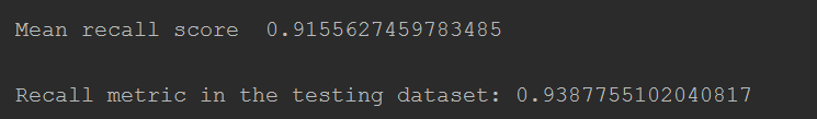
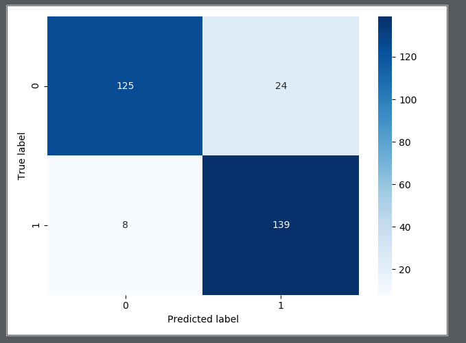
召回率也还可以,0.93多,但是由于采取的是下采样,样本数量是总样本的一部分,具有片面性。另外,发现有8个人,真实为1,预测为0,等于说没预测到。
best_c = printing_Kfold_scores(X_train, y_train)
输出如下:
------------------------------------------
C parameter: 0.1
-------------------------------------------

Iteration  1 : recall score =  0.5671641791044776
Iteration  2 : recall score =  0.6164383561643836
Iteration  3 : recall score =  0.6833333333333333
Iteration  4 : recall score =  0.5846153846153846
Iteration  5 : recall score =  0.525

Mean recall score  0.5953102506435158

------------------------------------------
C parameter: 1
-------------------------------------------

Iteration  1 : recall score =  0.5522388059701493
Iteration  2 : recall score =  0.6164383561643836
Iteration  3 : recall score =  0.7166666666666667
Iteration  4 : recall score =  0.6153846153846154
Iteration  5 : recall score =  0.5625

Mean recall score  0.612645688837163

------------------------------------------
C parameter: 10
-------------------------------------------

Iteration  1 : recall score =  0.5522388059701493
Iteration  2 : recall score =  0.6164383561643836
Iteration  3 : recall score =  0.7333333333333333
Iteration  4 : recall score =  0.6153846153846154
Iteration  5 : recall score =  0.575

Mean recall score  0.6184790221704963

------------------------------------------
C parameter: 100
-------------------------------------------

Iteration  1 : recall score =  0.5522388059701493
Iteration  2 : recall score =  0.6164383561643836
Iteration  3 : recall score =  0.7333333333333333
Iteration  4 : recall score =  0.6153846153846154
Iteration  5 : recall score =  0.575

Mean recall score  0.6184790221704963


Process finished with exit code 0
发现虽然下采样模型的recall比较高,但是用下采样的模型预测原始数据,recall才0.61多,所以存在局限性。
#再绘制混淆矩阵看看
lr = LogisticRegression(C=best_c, penalty='l1', solver='liblinear')
lr.fit(X_train, y_train.values.ravel())
y_pred = lr.predict(X_test.values)
y_pred = y_pred.tolist()
y_test = y_test['Class'].tolist()
cnf_matrix = confusion_matrix(y_test, y_pred)
print("Recall metric in the testing dataset:",
      cnf_matrix[1, 1] / (cnf_matrix[1, 0] + cnf_matrix[1, 1]))
#打印recall值
print('cnf_matrix[1, 1]=',cnf_matrix[1, 1],'cnf_matrix[1, 0]=',cnf_matrix[1, 0],'cnf_matrix[1, 1]=',cnf_matrix[1, 1])
plot_confusion_matrix(cnf_matrix)
plt.show()
输出混淆矩阵:
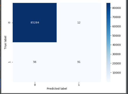
发现问题,如果从准确率的角度看,很高,但是从recall值看,很低,recall才0.61多。真实值为1的,预测值为0的,有56个人,这些人是检测不出来的。印证了刚才所说的下采样的片面性。
从另外一个角度讨论,如果修改预测0或1的阈值,结果怎么样?lr.predict函数默认阈值是0.5,如果修改阈值,需要使用lr.predict_proba函数。
lr = LogisticRegression(C=0.01, penalty='l1', solver='liblinear')
lr.fit(X_train_undersample, y_train_undersample.values.ravel())
y_pred_undersample_proba = lr.predict_proba(X_test_undersample.values)
#predict返回的是0或1,predict_proba返回的是0或1的概率值,所以y_pred_undersample_proba.shape=(296, 2)
#第0列是预测值为0的概率,第1列是预测值为1的概率。在这个背景下,预测结果只有0和1,在其他背景下,可能有0、1、2等等。
#所以每一行相加的概率值为1
thresholds = [0.1, 0.2, 0.3, 0.4, 0.5, 0.6, 0.7, 0.8, 0.9]  # 阈值列表
#目的是画出,不同阈值下的recall值和图像。比如阈值=0.1,大于0.1的意思是有10%的概率认为是确诊,就归为确定病例。
plt.figure(figsize=(10, 10)) #设定图的长宽
j = 1
for i in thresholds:  #遍历几种情况下的阈值
    y_test_predictions_high_recall = y_pred_undersample_proba[:, 1] > i
    # 如果预测的概率值大于阈值,就返回True,所以y_test_predictions_high_recall的值是一个bool型的list
    ax = plt.subplot(3, 3, j)  #设定子图画板
    ax.set_title('Threshold >= %s' % i)
    j += 1
    cnf_matrix = confusion_matrix(y_test_undersample,
                                  y_test_predictions_high_recall)
    print("Recall metric in the testing dataset:",
          cnf_matrix[1, 1] / (cnf_matrix[1, 0] + cnf_matrix[1, 1]))
    plot_confusion_matrix(cnf_matrix)
plt.show()
输出图像:

很容易看出来,阈值是0.5或0.6的情况下,recall值会好点。
再换种角度分析问题,既然下采样预测原始数据的效果不好,采用过采样呢?过采样就要增加样本数量,也就是Class=1的样本数量。
from imblearn.over_sampling import SMOTE
#导入SMOTE算法,第一次用需要安装,在anaconda Prompt下pip install imblearn就可以
credit_cards = pd.read_csv('creditcard.csv')
columns = credit_cards.columns
features_columns = columns.delete(len(columns) - 1)
features = credit_cards[features_columns]
labels = credit_cards['Class']
features['normAmount'] = StandardScaler().fit_transform(features['Amount'].values.reshape(-1,1))
print(features)
features = features.drop(['Time','Amount'],axis = 1)
print(features)
features_train, features_test, labels_train, labels_test = train_test_split(
    features, labels, test_size=0.2, random_state=0)
oversampler = SMOTE(random_state=0)
os_features,os_labels = oversampler.fit_sample(features_train,labels_train)
os_features = pd.DataFrame(os_features)
os_labels = pd.DataFrame(os_labels)
注意SMOTE.fit_sample(features_train,labels_train)
features_train:特征集
labels_train:标签集
该函数自动判断哪个是少数不平衡的类别,所以输入时将整体的训练集输入即可,不用将少数集预先提出。
输出:
------------------------------------------
C parameter: 0.01
-------------------------------------------

Iteration  1 : recall score =  0.8838709677419355
Iteration  2 : recall score =  0.8947368421052632
Iteration  3 : recall score =  0.9668916675888016
Iteration  4 : recall score =  0.9561886547740737
Iteration  5 : recall score =  0.9569360635737132

Mean recall score  0.9317248391567574

------------------------------------------
C parameter: 0.1
-------------------------------------------

Iteration  1 : recall score =  0.8838709677419355
Iteration  2 : recall score =  0.8947368421052632
Iteration  3 : recall score =  0.9688170853159235
Iteration  4 : recall score =  0.9586836812081644
Iteration  5 : recall score =  0.9592002725843858

Mean recall score  0.9330617697911343

------------------------------------------
C parameter: 1
-------------------------------------------

Iteration  1 : recall score =  0.8838709677419355
Iteration  2 : recall score =  0.8947368421052632
Iteration  3 : recall score =  0.9687064291247095
Iteration  4 : recall score =  0.9590683769138612
Iteration  5 : recall score =  0.9597498378782383

Mean recall score  0.9332264907528016

------------------------------------------
C parameter: 10
-------------------------------------------

Iteration  1 : recall score =  0.8838709677419355
Iteration  2 : recall score =  0.8947368421052632
Iteration  3 : recall score =  0.9689498727453801
Iteration  4 : recall score =  0.9591343247491234
Iteration  5 : recall score =  0.959486046537189

Mean recall score  0.9332356107757782

------------------------------------------
C parameter: 100
-------------------------------------------

Iteration  1 : recall score =  0.8838709677419355
Iteration  2 : recall score =  0.8947368421052632
Iteration  3 : recall score =  0.9689941352218656
Iteration  4 : recall score =  0.9588815247139513
Iteration  5 : recall score =  0.9595629856783284

Mean recall score  0.9332092910922688
从结果来看,每个惩罚系数都是差不多的。
lr = LogisticRegression(C = best, penalty = 'l1', solver='liblinear')
lr.fit(os_features,os_labels.values.ravel())
y_pred = lr.predict(features_test.values)
cnf_matrix = confusion_matrix(labels_test,y_pred)
plot_confusion_matrix(cnf_matrix)
plt.show()
输出的混淆矩阵:
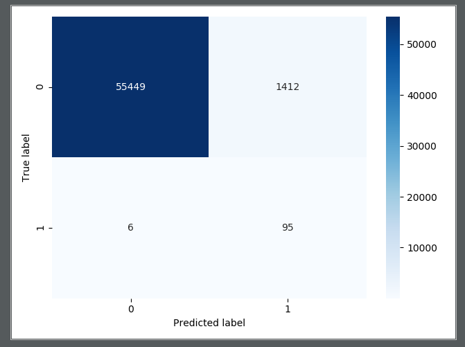
从输出的混淆矩阵来看,效果不错,至少recall=95/(95+6)=0.94多,只有6个人患病,但是没有预测到。比下采样好多了。
总结:除了学会处理样本不均衡的方法外,对于应用来说,不用过于关注算法具体如何实现的,只需要知道算法调用的函数名称、参数配置就可以。但是如果是写论文来说,想优化算法,就需要搞清楚算法的本质,用自己的代码去实现算法,再做优化。
本博客参考的是唐宇迪的机器学期视频,以及https://www.cnblogs.com/xiaoyh/p/11209909.html朋友的博客。

