TensorFlow文档翻译-01-TensorFlow入门

版权声明：本文为博主原创文章，转载请指明转载地址

http://www.cnblogs.com/junyang/p/7429771.html 

 

TensorFlow入门

英文原文地址：
https://www.tensorflow.org/get_started/get_started

这是关于如何开始tensorFlow的指南。开始之前，你需要先安装TensorFlow。除此之外，你应该了解：

• 知道如何使用Python编程。
• 懂一点点数组

如果具有机器学习的知识则更好。当然，如果你没有学习过机器学习，也应该先学习这个指引。

 

TensorFlow提供了很多的API。底层的API，是TensorFlow的核心，可以提供完整的控制功能，推荐希望对自己的模型进行更加细粒度控制的机器学习研究人员使用。高层次的API，建立在底层核心API之上，比底层核心API更加容易学习和使用，使用高层次的API可以更容易实现目标，并且适合不同水平的用户。高层的API比如 tf.estimator ，可以帮助你管理数据集，实现评估、训练、和推理。

本指南先是提供了一个TensorFlow  核心API的教程。然后，我们使用tf.estimator实现相同的模型。学习如何使用高层次API实现强大的功能。

 

Tensors – 张量

TensorFlow的核心数据单元是Tensor（张量），Tensor是存放基础类型数据的任意维度的数组。Rank（等级）即Tensor的维度数。以下是一些例子：

3 #一个等级为0的tensor，是一个标量其造型为[]
[1., 2., 3.] #等级为1的tensor，是一个矢量其造型为[3]
[[1., 2., 3.], [4., 5., 6.]] #等级为2的tensor,一个矩阵其造型为[2, 3]
[[[1., 2., 3.]], [[7., 8., 9.]]] #等级为3等tensor其造型为[2, 1, 3]

　

核心教程
导入TensorFlow，标准的导入TensorFlow库方式：

import tensorflow as tf

使得Python可以使用TensorFlow的类、方法和标识符。

 

 计算图（The Computational Graph）

你可能会认为TensorFlow核心程序包含两个独立两个部分：

1. 构建计算图
2. 运行计算图

计算图，即使用图形和节点的方式来标志TensorFlow系列操作安排。我们构建这样一个计算图，每个节点要么是0，要么是使用tensor数据为输入，tensor数据为输出。有一种节点的类型是常量，就像全部的TensorFlow的常量一样，它没有输入，并且他的输出内部存储的值。我们可以创建两个浮点型的节点，具体实现如下：

node1 = tf.constant(3.0, dtype=tf.float32)
node2 = tf.constant(4.0) # also tf.float32 implicitly
print(node1, node2)

　　

最后打印出来的结果是：

Tensor("Const:0", shape=(), dtype=float32) Tensor("Const_1:0", shape=(), dtype=float32)

　　

注意打印出来的节点并没有输出你期望的3.0和4.0数值，而是产生3.0和4.0的计算方式。如果想计算节点的值，需要使用session运行计算图。Session封装了TensorFlow运行时候的逻辑和状态。

下面的代码创建了session对象，并且调用了run方法执行计算图逻辑来计算node1和node2。运行代码如下：

sess = tf.Session()
print(sess.run([node1, node2]))

这个时候你会看到你期望的数值3.0和4.0：

[3.0, 4.0]

 

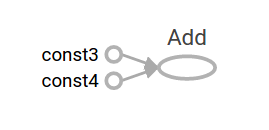
我们可以组合tensor阶段来构造更加复杂的计算，比如，我们可以让两个常量节点相加，得到的新的计算图：

node3 = tf.add(node1, node2)
print("node3:", node3)
print("sess.run(node3):", sess.run(node3))

　　

最后两行打印的结果是：

node3: Tensor("Add:0", shape=(), dtype=float32)
sess.run(node3): 7.0

TensorFlow 的工具TensorBoard能够显示计算图，这是一个TensorBoard的图形的例子：

 

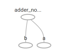
正如其表达的那样，计算图总是输出常量结果。使用占位符，计算图可以接收外部输入的参数。占位符是的我们可以在运行(run)时候提供具体的值。

a = tf.placeholder(tf.float32)
b = tf.placeholder(tf.float32)
adder_node = a + b  # 函数ft.add(a,b)的简写

这三行代码有点像一个函数或者lambda表达式，我们定义了两个参数（a和b），然后对其执行运算。我们输入不同的参数来执行运算，通过feed_dict 将参数传入实际值到占位符。

print(sess.run(adder_node, {a: 3, b: 4.5}))
print(sess.run(adder_node, {a: [1, 3], b: [2, 4]}))

　　

结果如下

7.5
[ 3.  7.]

　　

在TensorBoard中的图形是这样的：

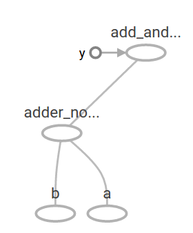
通过增加其他操作，我们可以让计算图更加复杂，比如：

add_and_triple = adder_node * 3.
print(sess.run(add_and_triple, {a: 3, b: 4.5}))

　　

结果如下

22.5

显示在TensorBoard中的计算图是这样的：

        

在机器学习中，我模型希望能够得到不同的输入，就如上面的例子。为了能够训练模型，我们需要修改计算图，使得在相同的输入情况下能够获取不同的输出。变量(variables) 允许我们增加训练参数到计算图中。构造变量时候需要提供类型和一个初始值：

W = tf.Variable([.3], dtype=tf.float32)
b = tf.Variable([-.3], dtype=tf.float32)
x = tf.placeholder(tf.float32)
linear_model = W * x + b

　　

常量在调用tf.constant时候初始化，常量的值不能被修改。相反的，变量在调用tf.Variable时候没有初始化。如果要初始化变量，你要调用一个特别的操作：

init = tf.global_variables_initializer()
sess.run(init)

 

要记住init方法是将初始化全部的全局变量的操作增加到TensorFlow的计算图中，并没有马上初始化变量。初始化的操作时在调用session.run时候进行的。

因为x是一个占位符，我们可以同时计算linear_mode的几个值：

print(sess.run(linear_model, {x: [1, 2, 3, 4]}))

输出如下：

[ 0.          0.30000001  0.60000002  0.90000004]

我们创建了model，但不知道模型的匹配程度有多好。为了使用训练数据评估模型，我们需要一个y 占位符去提供期望的值，并且要写一个损失函数。

损失函数计算当前的模型和实际的数据的差距情况。我们将使用一个标准的损失模型来做线性回归，计算当前模型和提供的数据之间的方差。Linear_model – y创建一个矢量，包含了每个样本和数据之间的偏差。调用ft.square得到偏差的平方值，使用tf.reduce_sum将全部的偏差的平方值加和存放到一个标量中。

y = tf.placeholder(tf.float32)
squared_deltas = tf.square(linear_model - y)
loss = tf.reduce_sum(squared_deltas)
print(sess.run(loss, {x: [1, 2, 3, 4], y: [0, -1, -2, -3]}))

得到和方差为：

23.66

　　

进一步改进，分别设置w和b的值为1和-1。变量开始时没有初始化的，除非调了用tf.variable时候进行的。但你也可以使用ft.assign来初始化了，比如，w=1和b=1是我们模型的优化参数，我们可以这样来修改w和b的值：

fixW = tf.assign(W, [-1.])
fixb = tf.assign(b, [1.])
sess.run([fixW, fixb])
print(sess.run(loss, {x: [1, 2, 3, 4], y: [0, -1, -2, -3]}))

　

最后输出的偏差是0：

0.0

完美的w和b的值是猜测出来的，但是我们希望机器学习能够自动的找出正确的参数，我们将会在下一个环节介绍。

 

tf.train API

完整的讨论机器学习已经超出了我们教程的范围。然而TensorFlow提供的优化器可以逐步的调整每个变量，来降低偏差。最简单的优化器是梯度下降优化器（gradient descent），它根据该变量的导数的偏差量级来调整每个变量。通常，手工计算导数非常无聊且容易出错。而使用tf.radients函数，TensorFlow能够帮你自动的计算导数。范例如下所示：

optimizer = tf.train.GradientDescentOptimizer(0.01)
train = optimizer.minimize(loss)

sess.run(init) # 重置其值为默认的值
for i in range(1000):
  sess.run(train, {x: [1, 2, 3, 4], y: [0, -1, -2, -3]})

print(sess.run([W, b]))

 

模型的参数最终如下：

[array([-0.9999969], dtype=float32), array([ 0.99999082],
 dtype=float32)]

　

虽然这个简单的线性回归不需要多少TensorFlow核心的代码，但现在我们正做在真正的机器学习的事情。更复杂的模型和方法要用更多的代码来提供数据。因为，为了便于使用，TensorFlow进一步抽象了通用的模式、架构和功能。我们会在下一个环节学习这些抽象。

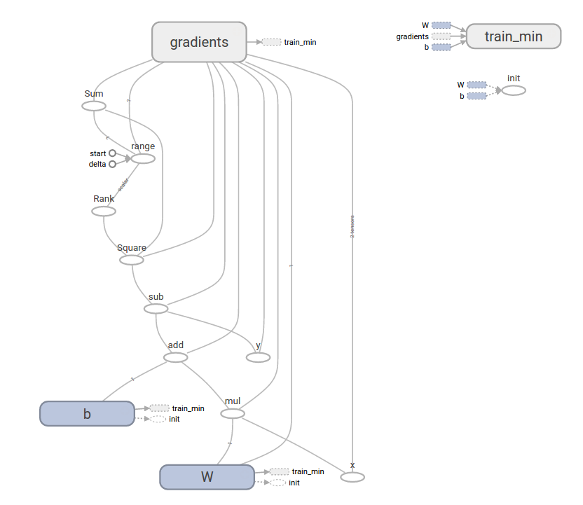
完整的线性回归模型训练如下：

import tensorflow as tf

#  模型的参数
W = tf.Variable([.3], dtype=tf.float32)
b = tf.Variable([-.3], dtype=tf.float32)
# Model input and output 模型的输入和输出
x = tf.placeholder(tf.float32)
linear_model = W * x + b
y = tf.placeholder(tf.float32)

# 偏差
loss = tf.reduce_sum(tf.square(linear_model - y)) # sum of the squares方差合计
# optimizer优化器
optimizer = tf.train.GradientDescentOptimizer(0.01)
train = optimizer.minimize(loss)

# 训练数据
x_train = [1, 2, 3, 4]
y_train = [0, -1, -2, -3]

# 循环训练
init = tf.global_variables_initializer()
sess = tf.Session()
sess.run(init) # reset values to wrong
for i in range(1000):
  sess.run(train, {x: x_train, y: y_train})

# 评估训练准确度
curr_W, curr_b, curr_loss = sess.run([W, b, loss], {x: x_train, y: y_train})
print("W: %s b: %s loss: %s"%(curr_W, curr_b, curr_loss))

　

运行后，结果如下：

W: [-0.9999969] b: [ 0.99999082] loss: 5.69997e-11

　　

注意到偏差已经是非常小的了（几乎等于0）。假如你运行这个程序，偏差可能会不一样，因为模型在初始化时候使用了伪随机的数值。

这个复杂的计算图仍然可以显示在TensorBoard中。 

tf.estimator

tf.estimator是一个高阶的TensorFlow库，可以简化机器学习过程，包括：

• 循环训练的运行
• 循环评估的运行
• 管理数据集

tf.estimator定义了很多通用的模型。

基本用法

注意，使用tf.estimator大大的简化了线性回归的过程：

import tensorflow as tf
# Numpy经常用来加载、控制和和预处理数据
import numpy as np

#声明变量，只有一个数字类型的变量
feature_columns = [tf.feature_column.numeric_column("x", shape=[1])]

#评估器在前端负责启动训练（装配）和评估（推论）。有许多预定义类型，如线性回归、线性分类、神经元网络分类器和回归器。
estimator = tf.estimator.LinearRegressor(feature_columns=feature_columns)


# TensorFlow提供很多协助函数来读取和设置数据集，在这里我们使用了2个数据集：一个用来训练，另一个用来做评估。我们要通知函数有几批数据（num_epochs）以及每批有多少的数据
x_train = np.array([1., 2., 3., 4.])
y_train = np.array([0., -1., -2., -3.])
x_eval = np.array([2., 5., 8., 1.])
y_eval = np.array([-1.01, -4.1, -7, 0.])
input_fn = tf.estimator.inputs.numpy_input_fn(
    {"x": x_train}, y_train, batch_size=4, num_epochs=None, shuffle=True)
train_input_fn = tf.estimator.inputs.numpy_input_fn(
    {"x": x_train}, y_train, batch_size=4, num_epochs=1000, shuffle=False)
eval_input_fn = tf.estimator.inputs.numpy_input_fn(
    {"x": x_eval}, y_eval, batch_size=4, num_epochs=1000, shuffle=False)

#在调用方法时候，传入训练训练数据集进行1000次的训练。
estimator.train(input_fn=input_fn, steps=1000)

# 在这里评估模型的执行情况
train_metrics = estimator.evaluate(input_fn=train_input_fn)
eval_metrics = estimator.evaluate(input_fn=eval_input_fn)
print("train metrics: %r"% train_metrics)
print("eval metrics: %r"% eval_metrics)

　　

运行的结果如下：

train metrics: {'loss': 1.2712867e-09, 'global_step': 1000}
eval metrics: {'loss': 0.0025279333, 'global_step': 1000}

注意运算结果显示更高的偏差，但是仍然接近0。意味着我们的机器学习是恰当的。

 

 自定义模型

tf.estimator并没有把你限制在定义好的模型中。假如你要创建一个自定义的、TensorFlow没有的模型。我们仍然可以使用tf.estimator的高级别的抽象，进行数据传送、训练等。在这里，我们通过低级别的TensorFlow的API，实现自己的和LinearRegressor一样的模型，

自定义的模型需要依赖tf.estimator来实现，我们要使用tf.estimator.Estimator。而tf.estimator.LinearRegressor实际是tf.estimator.Estimator的一个子类。我们使用Estimator的函数mode_fn通知ft.estimator 怎样的评估计算结果、训练步骤以及偏差。

代码如下：

import numpy as np
import tensorflow as tf

# Declare list of features, we only have one real-valued feature
def model_fn(features, labels, mode):
  # Build a linear model and predict values
  W = tf.get_variable("W", [1], dtype=tf.float64)
  b = tf.get_variable("b", [1], dtype=tf.float64)
  y = W * features['x'] + b
  # Loss sub-graph
  loss = tf.reduce_sum(tf.square(y - labels))
  # Training sub-graph
  global_step = tf.train.get_global_step()
  optimizer = tf.train.GradientDescentOptimizer(0.01)
  train = tf.group(optimizer.minimize(loss),
                   tf.assign_add(global_step, 1))
  # EstimatorSpec connects subgraphs we built to the
  # appropriate functionality.
  return tf.estimator.EstimatorSpec(
      mode=mode,
      predictions=y,
      loss=loss,
      train_op=train)

estimator = tf.estimator.Estimator(model_fn=model_fn)
# define our data sets
x_train = np.array([1., 2., 3., 4.])
y_train = np.array([0., -1., -2., -3.])
x_eval = np.array([2., 5., 8., 1.])
y_eval = np.array([-1.01, -4.1, -7, 0.])
input_fn = tf.estimator.inputs.numpy_input_fn(
    {"x": x_train}, y_train, batch_size=4, num_epochs=None, shuffle=True)
train_input_fn = tf.estimator.inputs.numpy_input_fn(
    {"x": x_train}, y_train, batch_size=4, num_epochs=1000, shuffle=False)
eval_input_fn = tf.estimator.inputs.numpy_input_fn(
    {"x": x_eval}, y_eval, batch_size=4, num_epochs=1000, shuffle=False)

# train
estimator.train(input_fn=input_fn, steps=1000)
# Here we evaluate how well our model did.
train_metrics = estimator.evaluate(input_fn=train_input_fn)
eval_metrics = estimator.evaluate(input_fn=eval_input_fn)
print("train metrics: %r"% train_metrics)
print("eval metrics: %r"% eval_metrics)

　　

运行结果：

train metrics: {'loss': 1.227995e-11, 'global_step': 1000}
eval metrics: {'loss': 0.01010036, 'global_step': 1000}

请注意自定义的model_fn函数的内容，和指南上的低层API的模型循环训练是很类似的。

 

Next steps 下一步骤

现在你具备TensorFlow的知识可以做一点事情了。我们还有好几个教程等着你去学习。假如你是机器学习的小白，可以先从MNIST for beginners开始学习，如果不是则可以直接学习 Deep MNIST for experts.。

Except as otherwise noted, the content of this page is licensed under the Creative Commons Attribution 3.0 License, and code samples are licensed under the Apache 2.0 License. For details, see our Site Policies. Java is a registered trademark of Oracle and/or its affiliates.

Last updated 八月 17, 2017.