Apache Spark源码走读之22 -- 浅谈mllib中线性回归的算法实现

欢迎转载，转载请注明出处，徽沪一郎。

概要

本文简要描述线性回归算法在Spark MLLib中的具体实现，涉及线性回归算法本身及线性回归并行处理的理论基础，然后对代码实现部分进行走读。

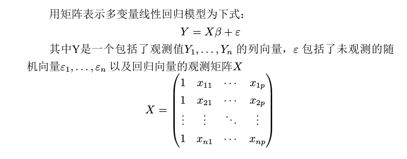
线性回归模型

机器学习算法是的主要目的是找到最能够对数据做出合理解释的模型，这个模型是假设函数，一步步的推导基本遵循这样的思路

假设函数
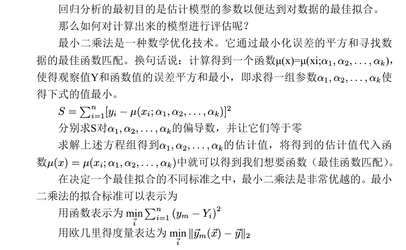
为了找到最好的假设函数，需要找到合理的评估标准，一般来说使用损失函数来做为评估标准
根据损失函数推出目标函数
现在问题转换成为如何找到目标函数的最优解，也就是目标函数的最优化

具体到线性回归来说，上述就转换为

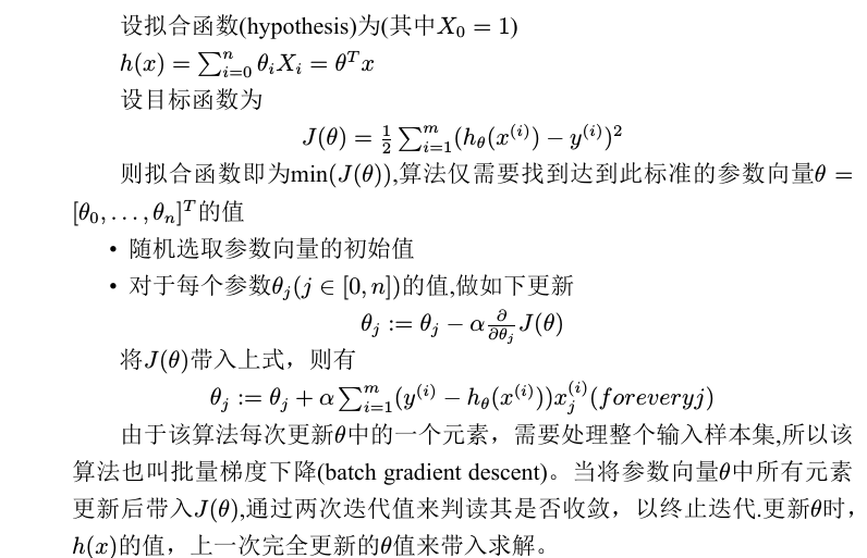
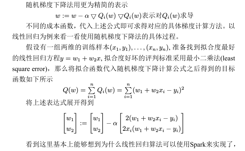
梯度下降法

那么如何求得损失函数的最优解，针对最小二乘法来说可以使用梯度下降法。

算法实现

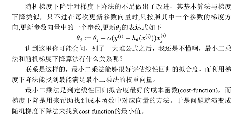
随机梯度下降

正则化

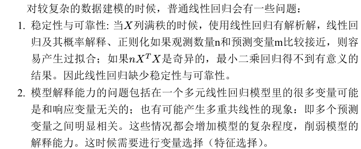
如何解决这些问题呢？可以采用收缩方法(shrinkage method)，收缩方法又称为正则化(regularization)。主要是岭回归(ridge regression)和lasso回归。通过对最小二乘估计加入罚约束,使某些系数的估计为0。

线性回归的代码实现

上面讲述了一些数学基础，在将这些数学理论用代码来实现的时候，最主要的是把握住相应的假设函数和最优化算法是什么，有没有相应的正则化规则。

对于线性回归，这些都已经明确，分别为

Y = A*X + B 假设函数
随机梯度下降法
岭回归或Lasso法，或什么都没有

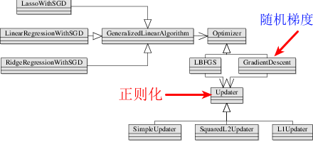
那么Spark mllib针对线性回归的代码实现也是依据该步骤来组织的代码，其类图如下所示

函数调用路径

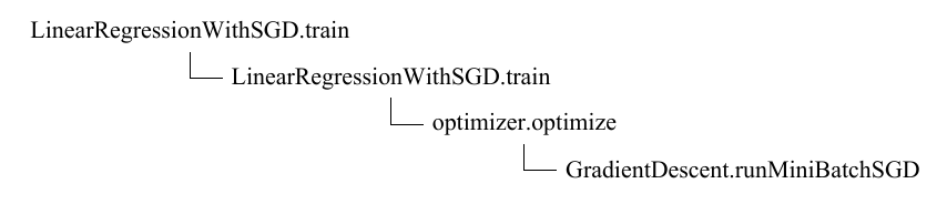
train->run,run函数的处理逻辑

利用最优化算法来求得最优解,optimizer.optimize
根据最优解创建相应的回归模型, createModel

runMiniBatchSGD是真正计算Gradient和Loss的地方

def runMiniBatchSGD(
      data: RDD[(Double, Vector)],
      gradient: Gradient,
      updater: Updater,
      stepSize: Double,
      numIterations: Int,
      regParam: Double,
      miniBatchFraction: Double,
      initialWeights: Vector): (Vector, Array[Double]) = {

    val stochasticLossHistory = new ArrayBuffer[Double](numIterations)

    val numExamples = data.count()
    val miniBatchSize = numExamples * miniBatchFraction

    // if no data, return initial weights to avoid NaNs
    if (numExamples == 0) {

      logInfo("GradientDescent.runMiniBatchSGD returning initial weights, no data found")
      return (initialWeights, stochasticLossHistory.toArray)

    }

    // Initialize weights as a column vector
    var weights = Vectors.dense(initialWeights.toArray)
    val n = weights.size

    /**
     * For the first iteration, the regVal will be initialized as sum of weight squares
     * if it's L2 updater; for L1 updater, the same logic is followed.
     */
    var regVal = updater.compute(
      weights, Vectors.dense(new Array[Double](weights.size)), 0, 1, regParam)._2

    for (i  (c, v) match { case ((grad, loss), (label, features)) =>
            val l = gradient.compute(features, label, bcWeights.value, Vectors.fromBreeze(grad))
            (grad, loss + l)
          },
          combOp = (c1, c2) => (c1, c2) match { case ((grad1, loss1), (grad2, loss2)) =>
            (grad1 += grad2, loss1 + loss2)
          })

      /**
       * NOTE(Xinghao): lossSum is computed using the weights from the previous iteration
       * and regVal is the regularization value computed in the previous iteration as well.
       */
      stochasticLossHistory.append(lossSum / miniBatchSize + regVal)
      val update = updater.compute(
        weights, Vectors.fromBreeze(gradientSum / miniBatchSize), stepSize, i, regParam)
      weights = update._1
      regVal = update._2
    }

    logInfo("GradientDescent.runMiniBatchSGD finished. Last 10 stochastic losses %s".format(
      stochasticLossHistory.takeRight(10).mkString(", ")))

    (weights, stochasticLossHistory.toArray)

  }

上述代码中最需要引起重视的部分是aggregate函数的使用,先看下aggregate函数的定义

def aggregate[U: ClassTag](zeroValue: U)(seqOp: (U, T) => U, combOp: (U, U) => U): U = {
    // Clone the zero value since we will also be serializing it as part of tasks
    var jobResult = Utils.clone(zeroValue, sc.env.closureSerializer.newInstance())
    val cleanSeqOp = sc.clean(seqOp)
    val cleanCombOp = sc.clean(combOp)
    val aggregatePartition = (it: Iterator[T]) => it.aggregate(zeroValue)(cleanSeqOp, cleanCombOp)
    val mergeResult = (index: Int, taskResult: U) => jobResult = combOp(jobResult, taskResult)
    sc.runJob(this, aggregatePartition, mergeResult)
    jobResult
  }

aggregate函数有三个入参,一是初始值ZeroValue,二是seqOp,三为combOp.

seqOp seqOp会被并行执行,具体由各个executor上的task来完成计算
combOp combOp则是串行执行, 其中combOp操作在JobWaiter的taskSucceeded函数中被调用

为了进一步加深对aggregate函数的理解,现举一个小小例子。启动spark-shell后,运行如下代码

val z = sc. parallelize (List (1 ,2 ,3 ,4 ,5 ,6),2)
z.aggregate (0)(math.max(_, _), _ + _)
// 运 行 结 果 为 9
res0: Int = 9

仔细观察一下运行时的日志输出, aggregate提交的job由一个stage(stage0)组成,由于整个数据集被分成两个partition,所以为stage0创建了两个task并行处理。

LeastSquareGradient

讲完了aggregate函数的执行过程, 回过头来继续讲组成seqOp的gradient.compute函数。

LeastSquareGradient用来计算梯度和误差,注意cmopute中cumGraident会返回改变后的结果。这里计算公式依据的就是cost-function中的▽Q(w)

class LeastSquaresGradient extends Gradient {
  override def compute(data: Vector, label: Double, weights: Vector): (Vector, Double) = {
    val brzData = data.toBreeze
    val brzWeights = weights.toBreeze
    val diff = brzWeights.dot(brzData) - label
    val loss = diff * diff
    val gradient = brzData * (2.0 * diff)

    (Vectors.fromBreeze(gradient), loss)
  }

  override def compute(
      data: Vector,
      label: Double,
      weights: Vector,
      cumGradient: Vector): Double = {
    val brzData = data.toBreeze
    val brzWeights = weights.toBreeze
    //dot表示点积，是接受在实数R上的两个向量并返回一个实数标量的二元运算，它的结果是欧几里得空间的标准内积。
    //两个向量的点积写作a·b。点乘的结果叫做点积，也称作数量积
    val diff = brzWeights.dot(brzData) - label

    //下面这句话完成y += a*x
    brzAxpy(2.0 * diff, brzData, cumGradient.toBreeze)

    diff * diff
  }
}

在上述代码中频繁出现breeze相关的函数,你一定会很好奇,这是个什么新鲜玩艺。

说开了其实一点也不稀奇, 由于计算中有大量的矩阵(Matrix)及向量(Vector)计算,为了更好支持和封装这些计算引入了breeze库。

Breeze, Epic及Puck是scalanlp中三大支柱性项目, 具体可参数www.scalanlp.org

正则化过程

根据本次迭代出来的梯度和误差对权重系数进行更新,这个时候就需要用上正则化规则了。也就是下述语句会触发权重系数的更新

  val update = updater.compute(
     weights, Vectors.fromBreeze(gradientSum / miniBatchSize), stepSize, i, regParam)

以岭回归为例，看其更新过程的代码实现。

class SquaredL2Updater extends Updater {
  override def compute(
      weightsOld: Vector,
      gradient: Vector,
      stepSize: Double,
      iter: Int,
      regParam: Double): (Vector, Double) = {
    // add up both updates from the gradient of the loss (= step) as well as
    // the gradient of the regularizer (= regParam * weightsOld)
    // w' = w - thisIterStepSize * (gradient + regParam * w)
    // w' = (1 - thisIterStepSize * regParam) * w - thisIterStepSize * gradient
    val thisIterStepSize = stepSize / math.sqrt(iter)
    val brzWeights: BV[Double] = weightsOld.toBreeze.toDenseVector
    brzWeights :*= (1.0 - thisIterStepSize * regParam)
    brzAxpy(-thisIterStepSize, gradient.toBreeze, brzWeights)
    val norm = brzNorm(brzWeights, 2.0)

    (Vectors.fromBreeze(brzWeights), 0.5 * regParam * norm * norm)
  }
}

结果预测

计算出权重系数(weights)和截距intecept，就可以用来创建线性回归模型LinearRegressionModel，利用模型的predict函数来对观测值进行预测

class LinearRegressionModel (
    override val weights: Vector,
    override val intercept: Double)
  extends GeneralizedLinearModel(weights, intercept) with RegressionModel with Serializable {

  override protected def predictPoint(
      dataMatrix: Vector,
      weightMatrix: Vector,
      intercept: Double): Double = {
    weightMatrix.toBreeze.dot(dataMatrix.toBreeze) + intercept
  }
}

注意LinearRegression的构造函数需要权重(weights)和截距(intercept)作为入参，对新的变量做出预测需要调用predictPoint

一个完整的示例程序

在spark-shell中执行如下语句来亲自体验一下吧。

import org.apache.spark.mllib.regression.LinearRegressionWithSGD
import org.apache.spark.mllib.regression.LabeledPoint
import org.apache.spark.mllib.linalg.Vectors

// Load and parse the data
val data = sc.textFile("mllib/data/ridge-data/lpsa.data")
val parsedData = data.map { line =>
  val parts = line.split(',')
  LabeledPoint(parts(0).toDouble, Vectors.dense(parts(1).split(' ').map(_.toDouble)))
}

// Building the model
val numIterations = 100
val model = LinearRegressionWithSGD.train(parsedData, numIterations)

// Evaluate model on training examples and compute training error
val valuesAndPreds = parsedData.map { point =>
  val prediction = model.predict(point.features)
  (point.label, prediction)
}
val MSE = valuesAndPreds.map{case(v, p) => math.pow((v - p), 2)}.mean()
println("training Mean Squared Error = " + MSE)

小结

再次强调，找到对应的假设函数，用于评估的损失函数，最优化求解方法，正则化规则

posted @ 2014-08-15 20:04 徽沪一郎阅读(4843) 评论(3) 编辑收藏举报

会员力量，点亮园子希望

刷新页面返回顶部